Elm Wealth Research

Posts by:

James White

Is Vanguard More Rolls Royce, or Hyundai?

July 17, 2018

Featured Insights

Is Vanguard More Rolls Royce, or Hyundai?

By Victor Haghani and James White 1

“What we obtain too cheap, we esteem too lightly.”
  – Thomas Paine, 1776

A physician thinking about investing with Elm asked us: “If I hurt my knee, I’m going to find the best orthopedic surgeon available and I’ll expect to happily pay top dollar. Why is hiring an investment manager any different?”

Great question.

Alas, identifying the “best” investment managers isn’t so easy. Daniel Kahneman discusses this in “Thinking Fast and Slow”, asking the question “When can you trust an experienced professional who claims to have an intuition?” His answer is that the skill we are looking for should develop “through prolonged practice” in “an environment that is sufficiently regular to be predictable…[and providing] immediate and unambiguous feedback.” Many (if not most) crafts provide an excellent environment for developing unambiguous expertise, and it’s reasonable to expect to pay more for accessing that evident expertise.

Not so with investing; it’s hard to imagine a domain more irregular, unpredictable and ambiguous. And not only is it challenging for investment managers to consistently develop such unambiguous skill, but for the consumer, it is very difficult to distinguish true skill from good luck with the amount of historical data typically available to investors.2 In our paper What’s Past is Not Prologue, we suggested that even 20 years of historical performance data isn’t normally enough to distinguish with high confidence between skilled and average mutual fund managers.

Investment products aren’t the only ones whose merits are difficult for consumers to assess. However, with most other products, better quality normally goes hand-in-hand with a higher price, and so we can use price as a filter to narrow down the choices when trying to find the best service or product. For example, at Elm we recently upgraded one of our laptops. We needed a higher-performance machine, and it was pretty easy to know how to identify one: we looked for higher-price laptops, and we were quickly able to narrow the options down to the few best. This heuristic doesn’t work with hiring investment managers though – partly because the difficulty of judging skill hinders price efficiency, and partly because the quality of the product and the price paid in fees are not ‘separable.’

When buying a car, the car’s quality and the money you pay for it are separable. A very wealthy person (or an extreme car enthusiast) might pay 10 times the price of a standard car for one which is only 10% better, and still be happy with their decision. Investing is different from most other consumer choices in that what you get and what you pay both come in the form of dollars, so they’re not separable. “What you get” is risk-adjusted excess return in dollars, and “what you pay” are the fees in dollars. No matter how wealthy a person is, she will never knowingly pay $2 to get $1 of extra wealth.3

The uncertainty surrounding the “what you get” part of investment services can pave the way for us to unknowingly make a wealth-reducing exchange. In choosing a doctor, even if we fail to find the best doctor, an average doctor with the relevant medical qualifications is still pretty likely to do a good job. However, as we know from Sharpe’s “Arithmetic of Active Management,” the zero-sum nature of the investing game means the average investment manager is expected to deliver below average results.

Despite all these obstacles, many investors and their advisors still persevere against the odds in the quest of identifying the “best” investment managers. Behavioral economists would explain this by citing our natural tendency to over-extrapolate from small samples of data, combined with our proclivity to be overconfident in our abilities and decision-making.

Bill McNabb, former CEO of the Vanguard Group, explains that many of our consumer instincts about price and value lead us astray when it comes to choosing investment products:

“The whole cost argument from an investment perspective is counter-intuitive. If you think about your life in other areas, if you are out buying a car, you can buy a Rolls Royce and pay whatever Rolls Royces are going for today, or you can buy an inexpensive Hyundai. You are going to feel a difference in the car. Now whether it is worth it…only you as a buyer can make that decision. But, you are definitely going to feel the difference in quality. In investing, that equation doesn’t hold. And so, when you think about the average investor who is also a consumer, they are used to – the more I pay the higher the quality, the better the results I get. You come to investing and it is just the opposite.4 I think that it is really a hard behavior for people to unlearn.”5

But to improve as investors, unlearn we must.


  1. Victor is the Founder and CIO of Elm Partners, and James is Elm’s CEO. Past returns are not indicative of future performance. This not is not an offer or solicitation to invest.
  2. This is not true for all track records and all situations, but it is true often enough.
  3. Of course, in the context of investing, the equation is rarely so clear: “what you get” is, more formally, expected marginal utility in the context of your whole portfolio, and this is not directly observable. Historical net returns may be informative in this regard, but are still an imperfect proxy.
  4. To wit, McNabb cited a recent Morningstar study which found that, “A fund’s annual fee is the most proven predictor of future fund returns.” http://www.morningstar.co.uk/uk/news/149421/how-fund-fees-are-the-best-predictor-of-returns.aspx
  5. Watch: https://www.youtube.com/watch?v=SwkjqGd8NC4, starting at 43:16.
Read More

A Penny Saved is Two Pennies Earned

April 6, 2018

Investing 101

A Penny Saved is Two Pennies Earned

By Victor Haghani and James White 1

Most of us associate the maxim “A penny saved is a penny earned” with Benjamin Franklin, but what he actually said is far more insightful: “A penny saved is two pence clear”. By the time he penned this, in “Hints for Those That Would be Rich” of the 1737 Poor Richard’s Almanac, Franklin was an experienced businessman who understood the nature of risk and uncertainty. Although he didn’t elaborate on this pithy bit of advice, we think that he was trying to convey an idea much more profound than the simple identity expressed in the misquote. We believe he was getting at the notion that one risk-free penny saved is worth two pennies of expected but uncertain business income.

Ben Franklin was a man well ahead of his time: it wasn’t until about 230 years later that Paul Samuelson and Robert Merton arrived at the same conclusion using the tools of mathematical finance.2 Starting with the standard set of assumptions3 of a risk-averse investor and a single risky asset, they showed that if the investment in the risky asset is “perfectly” sized, the investor should be equally happy with a riskless investment delivering half the expected excess return of the investment in the risky asset.4 We could also say that under these circumstances, the investment’s “risk-adjusted return” is equal to half its expected excess return.

When Fees Saved are Worth More than Uncertain Extra Expected Return

One intriguing implication of this idea is that 1% more in investment management fees requires more than 1% in extra expected return, if getting the extra expected return increases the risk the investor is bearing. Just how much extra expected return an investor needs in order to offset the certain cost of higher fees depends on how much extra risk the manager has to take. For example, say an investor is considering moving from an index fund into an actively managed fund that charges 1% more in fees. Also assume that the index fund has a risk of 16%, but the active fund has a higher risk of 19% because it’s trying to generate higher returns by holding a more concentrated portfolio of stocks. In this case, the active fund needs to have a pre-fee expected return about 2% higher than the index fund to make the investor indifferent between the index fund and the active fund, a modern-day illustration of Franklin’s maxim.5

Conclusion

Philadelphia’s most famous resident tirelessly promoted the virtues of efficiency and rational thought which contributed so much to America’s economic success. It’s inspiring to realize that some of his ideas wound up being proven correct using mathematical techniques developed over 200 years later. Ben Franklin was a successful entrepreneur and his insight about the relative value of risky versus risk-free sources of return was developed in that light, but we see that it still has high practical value today for investors and business owners alike.


Appendix: A Slightly Deeper Dive

If we start with a risky portfolio which follows a geometric random walk,6 and then graph the relationship between Expected Excess Return, Risk-Adjusted Return, and the Price of Risk, it looks like this:

As the fraction of wealth invested in the risky portfolio increases, Expected Excess Return goes up in a straight line, while Risk-Adjusted Return goes up, peaks, then goes back down as risk starts to dominate. The optimal holding is the holding which maximizes Risk-Adjusted Return, or an allocation of 50% of wealth in this example.

Now we can also see that at the 50% point, Risk-Adjusted Return looks like it’s about half of the Expected Excess Return. In fact, it’s exactly half. In the theory of financial decision-making under uncertainty pioneered by Samuelson, Merton et al., there’s a result that within a standard set of assumptions the optimal Risk-Adjusted Return will always equal half of the Expected Excess Return at that optimal wealth allocation.7

So, to get one cent worth of Risk-Adjusted Return, the investor – regardless of their level of risk-aversion – would need two cents of Expected Excess Return if their wealth is optimally allocated. Risk-adjusted Return can be thought of as the risk-free return equivalent to the Expected Excess Return,8 so at the optimal allocation point we have a 2:1 ratio between the “risky” Expected Excess Return and the equivalent risk-free return.


  1. Victor is the Founder and CIO of Elm Partners, and James is Elm’s CEO. Past returns are not indicative of future performance. This not is not an offer or solicitation to invest.
     

    Thank you to Larry Hilibrand, Vlad Ragulin and Jeff Rosenbluth for their helpful comments.

  2. Samuelson and Merton weren’t the only ones or the first who arrived at this conclusion, but theirs is perhaps the most general formulation. See Robert C. Merton, “Lifetime Portfolio Selection under Uncertainty: the Continuous-Time Case,” The Review of Economics and Statistics (51), 1969, here.
  3. The standard set of assumptions are that the portfolio consists of a single risky asset following Geometric Brownian Motion, the portfolio is continuously re-balanced, interest rates are constant, and the investor’s risk-aversion is consistent with iso-elastic utility (Constant Relative Risk-Aversion).
  4. Where “perfectly” sized means sized to deliver optimal expected utility or optimal risk-adjusted return, and “equally happy” means to derive equal expected utility or equal risk-adjusted return.
  5. In general, the relationship between fees and extra expected return needed to make the investor equally well-off will vary, as it is a function of how much extra risk the higher fee investment needs to take on to deliver the extra expected return. The lower the extra risk, the smaller the ratio will be (and if the higher fee investment has a lower risk, it can have a lower expected excess return).
     

    Also, the example assumes that the investor will move his holding to a new optimal asset allocation reflecting the new risk and return characteristics of the actively managed investment. The ratio between $1 of risk-free marginal return and the equivalent risky expected excess return may not be exactly 2:1 as in our stylized example, but it is generally valid that we should give extra weight to a source of risk-free return- the penny saved- compared to a risky source of extra expected return- the two pennies earned.

  6. And the investor has a standard form of risk-aversion (CRRA), and re-balances the portfolio continuously.
  7. For a more detailed mathematical treatment, see Appendix C of our note here.
  8. Because an investment with a 1% risk-free return will also have a 1% Risk-Adjusted Return.
Read More

Sensible Investing in a Nutshell: Robin Powell, The Evidence-Based Investor, interviews Victor

March 12, 2018

In the News

Sensible Investing in a Nutshell: Robin Powell, The Evidence-Based Investor, interviews Victor

In this five-minute video Robin Powell, aka the Evidence-Based Investor, interviews Victor in his “journey to uncover the truth behind investing”. They discuss the meaning of the Puzzle of the Missing Billionaires and explore some of the reasons why investors don’t get the returns they should earn. The interview ends with Robin asking Victor: “What then would you advise young investors to do?”

Robin Powell is an award-winning financial journalist, blogger and educator in the field of investing. For the past six years, under the mantle of The Evidence-Based Investor, he has campaigned for better investor education and for greater transparency in global asset management. Prior to that, he reported for ITV and Sky News for over 20 years, after receiving his BA/MA in History from Oxford.


Disclaimer:

This video does not constitute investment advice. Past returns may not be indicative of future returns.

Read More

What Gamblers Can Teach the Buy-and-Hold Crowd

February 26, 2018

Risk and Return

What Gamblers Can Teach the Buy-and-Hold Crowd

By Victor Haghani and James White 1

The ongoing attack on stock-picking waged over the past 65 years now clearly has the upper hand. Early combatants included Markowitz, Samuelson, Sharpe, Fama, and Bogle, and as testament to their success it has become part of the conventional wisdom that ordinary investors should invest primarily in highly diversified, low cost, tax efficient index funds.

It’s become almost a corollary to this view that market-timing is also a fool’s errand; investors can’t hope to beat the market by predicting if the market is going to go up or down in the next day, month or year. Authors such as Burton Malkiel, through his influential book “A Random Walk Down Wall Street”, have argued that the Efficient Market Hypothesis, and its attendant Random Walk Hypothesis, mean that investors can only expect to hurt themselves by market timing. Many financial advisers, human and robotic, follow this line, recommending that investors should choose a level of stock market investment they are comfortable with and stick to it for the long term.2

The cases against stock-picking and market-timing seem to be pointing in the same direction: an investor can’t reasonably expect to beat the market. On closer inspection though, these activities have meaningful differences. Stock picking is largely a zero-sum activity dependent on market inefficiency. What one stock picker makes relative to the market must be the loss of another with the offsetting overweight and underweight portfolio holdings. In contrast, varying one’s exposure to the market is not zero-sum and need not rely on market inefficiency, as we’ll explore further below. One investor increasing her exposure doesn’t necessarily require a reduction from another. In fact, all investors can increase or decrease their exposure at the same time, either through a change in the price of the stock market,3 or through a change in the amount of equities outstanding. Rather than being a ‘bet’ versus the market or another investor, one investor’s optimal level of market exposure is a matter of how much risk is right for that investor given her forecast of the reward and risk of the market and her personal level of risk aversion.

The investing and gambling literature has long supported the idea that investors should change their exposure as their expectations4 of return and risk change. The Merton Rule in investing and the closely related Kelly Criterion in gambling are formal models of an entirely common-sense concept: the amount of savings we should optimally expose to the favorable but uncertain gamble of investing in the stock market should vary in proportion to expected return, and in inverse proportion to risk and our level of risk aversion.5 Under this model, the proposition that investors should hold a constant market exposure requires that either the expected excess return remains constant through time, or that the risk/reward ratio stays constant.6

Let’s focus first on expected excess return. Most researchers and practitioners would tell us the expected excess return of the stock market isn’t constant. For example, Yale Professor Robert Shiller has shown that the Cyclically-Adjusted Price to Earnings (CAPE) ratio of the stock market is a decent predictor of long-term real stock market returns, as shown in the chart below.7 Note that the return data as a function of CAPE is not primarily a result of the mean-reversion of CAPE; rather it is mostly explained by the starting earnings yield of the market, much as the 10-year return on a 10-year bond is almost entirely predicted by the bond’s yield-to-maturity at the time of purchase.8 And CAPE is just one of a number of indicators that can be used to form our expectation for the future return of the stock market, without relying on historical averages or reversion to a “fair” or average level.9

Ask yourself if you would have expected the US stock market to deliver the same long-term real return starting in 1985 when the US stock market CAPE was 10x as what it would deliver from 1965 when the CAPE was 23x?10 If you agree the lower CAPE in 1985 predicted higher expected real returns than the higher CAPE prevailing in 1965, then ex-ante, all else equal, you would have wanted a greater equity exposure in 1985 vs. 1965.11 And indeed your expectation would have been correct, as over the subsequent 30 years the real return of the US stock market was 8.2% from 1985 but only 4.2% from 1965.12

Believing that the expected excess return of the stock market changes over time is not at odds with a belief in market efficiency. Just like the price of milk and eggs, the expected aggregate real returns available in the market are a function of supply and demand, in particular the supply of investments and the demand from savers. As this supply/demand dynamic changes over time, so too do expected market returns, even in the perfectly efficient markets imagined by financial theorists.

Next, do we think it’s reasonable to assume the stock market’s risk/reward ratio stays constant? It seems plausible that an increase in expected return would be accompanied by, or maybe even caused by, an increase in expected risk.13 But while it is plausible it is not required, nor do we think it likely that such changes in risk exactly offset changes in expected return to leave the risk/reward ratio constant. For example, while expected returns were very different from the starting points of 1965 and 1985, as detailed above, the realized stock market risk over the two ensuing 30-year periods was virtually the same. Indeed, there is no theoretical reason to presume this ratio wouldn’t change over time. In fact, theory tells us that, for a given amount of savings, if there was a net issuance of new equity we should expect returns to go up without a material change to risk.

Critics of variable investment sizing point to the historical record to show that an investor would have been better off keeping a fixed fraction of their portfolio invested in equities rather than varying it based on a forward-looking, expected return predictor.14 In the Appendix, we show that a more careful look at the past 118 years of U.S. experience does not support that claim. By basing our analysis on the Merton Rule, we also counter the argument that back-tests of variable asset allocation require knowing the CAPE average in advance. We have put this analysis into the Appendix because we believe that expectations-driven sizing stands on its own logic, and that the limited US stock market history, while supportive, should not be taken as the primary reason to follow this approach.

When we look back to assess whether we’ve been well-served by following an expectations-driven approach, we must be careful to view outcomes not solely on how much we have grown our wealth, but also take account of how much risk we have taken along the way. To illustrate what we mean, imagine you are presented with the opportunity to bet on a coin that has a 70% chance of landing heads. You determine you want to bet 20% of your wealth on each flip.15 Then you are told that this coin is being replaced with a coin that has a 60% chance of landing heads. You now change your betting fraction to only bet 10% of your wealth on each flip, which is the rational, Kelly-consistent thing to do. In the next 100 flips, 60 come up heads and 40 come up tails, exactly what you expected for a 60/40 coin. You calculate that if you had still been betting 20% of your wealth on each bet, you’d have more wealth. Did you make the wrong decision to reduce your betting size from 20% to 10% of your wealth? We suggest you did not, because there was a higher chance of a worse outcome, and you properly accounted for that risk by reducing your bet size accordingly. The appropriate risk-adjusted measure of return (as described in the Appendix) would show just that.

Conclusion

It’s time to dispense with the pejorative and fuzzy term “market-timing” in favor of a more precise and neutral description for the kind of systematic, proportional change in investment sizing embodied by rules such as the Merton Rule and Kelly Criterion. We propose “expectation-driven sizing”, though we admit that doesn’t quite roll off the tongue.16

We’ve tried to show that variable, expectation-driven asset allocation is both theoretically sound and intuitively appealing. When the market offers lower expected returns, all else equal, it’s both good theory and good sense to own less of it. There’s a fundamental flaw in the prevailing conventional approach, in which the investor decides how much risk to take based solely on whether her individual level of risk aversion is above or below average, without factoring in how much she’s earning to take that risk. It would be like deciding to bet the same amount on a biased coin whether it’s 60/40 or 70/30 in your favor.

The goal of expectation-driven sizing is not for investors to beat the market, but rather to make the most of what the market is offering at each point in time, on a risk-adjusted basis. Somewhere along the road, this common-sense investing idea became confounded with the zero-sum proposition of trying to beat the market through stock-picking or short-term market speculation.17 It’s also true that “market-timing” has acquired a bad reputation in that that many investors have instead shown a tendency to vary their exposure to the market in an ad hoc, non-systematic manner, with bad results. Indeed, we agree it would be better to keep to a fixed exposure than to chase returns by varying one’s exposure based on a simple extrapolation of recent returns, or to put one’s faith in rapid reversion to some subjective assessment of fair value.

Bottom line: Investors should continue to employ low-cost, tax-efficient index funds and ETFs as the building blocks of their portfolios, and they should not be afraid to vary their exposure to the market in a disciplined fashion based on its expected attractiveness, which at Elm Partners is exactly what we mean by Active Index Investing®.


Appendix: A Closer Look at Static vs Expectations-Driven Sizing through 118 years of US Equity Market Experience

While the analysis below finds that an expectations-driven sizing of exposure to the U.S. equity market delivered superior risk-adjusted returns to a hypothetical investor under a given set of assumptions, we must stress that the past 118-year historical record of one stock market isn’t enough data to reach a statistically significant conclusion.

The table below compares the inflation-adjusted return an investor would have earned following:
1) a static, constant allocation of 65% in the S&P500 and 35% in US T-bills, or,
2) a return-driven, variable allocation between the S&P500 index and US T-bills, using the Merton rule for sizing.

Notice that expectation-driven sizing produces higher risk-adjusted real returns over the three periods considered in the table (see assumptions box below for how we calculate risk-adjusted returns). Of note is the most recent 18-year period starting with the year 2000, to which the critic of variable sizing might call our attention. Over this period, a static 65% allocation to equities produced a higher realized return than what an investor would have earned with the smaller allocation to equities called for by the Merton Rule. The reason for this is simple: over the past 18 years, CAPE has averaged 25.8x which indicated a low long-term expected excess return for equities, and hence it would have been sensible for a risk-averse investor to have a relatively small exposure to equities. Indeed, it transpired that the real return of US equities over the past 18 years was a relatively meager 4.79%. So, our investor who held less equities was justified ex-ante and ex-post in holding less equities, but we can only see this if we compare the risk-adjusted real return earned by the two strategies, not their gross returns. It is only by explicitly taking risk into account that we can see clearly that even though the investor who held less equities wound up with less wealth today, he was better off after taking risk into account, enjoying a real risk-adjusted return of 2.04% versus 1.30%.


Assumptions:

Data from Professor Robert Shiller’s website, from the start of 1900 to February 2018. Quarterly rebalancing using Merton Rule, with 1/CAPE for expected excess return on equities, hypothetical investor with CRRA utility with coefficient of risk aversion, η = 3 , assuming equity market volatility throughout of 18% pa, equity market follows geometric Brownian motion, 0 leverage allowed which was binding at different times (see chart above). For example, at CAPE = 16 , optimal equity allocation is 64%.

Risk-adjusted returns calculated by subtracting   η(ασ)22, where α is fraction of wealth invested in the stock market, σ = 18% , and η = 3 . We used 1/CAPE for the expected excess return of equities as we did not have a long-term forward-looking estimate of the real rate on the risk-free asset, and we feel that 1/CAPE is an under-estimate of long-term real returns of equities of about 1%, which we think would have been close to the long-term expected real rate since 1900.


  1. Victor is the Founder and CIO of Elm Partners, and James is Elm’s CEO. Past returns are not indicative of future performance. This not is not an offer or solicitation to invest.
     

    Thank you to Larry Hilibrand, Antti Ilmanen, Spencer Jakab, Arjun Krishnamachar, Bruce Lafranchi, Andy Morton, Vlad Ragulin, Jeff Rosenbluth and Rich Dewey for their very helpful comments and suggestions. A working draft of this note was discussed by John Authers in this Financial Times article.

  2. An exception to the strict rule allowed for reducing the allocation to equities in old age.
  3. As we discuss here.
  4. Throughout this note we use “expectation” and “expected” in the common-language sense, not in the sense of mathematical expectation.
  5. The Kelly Criterion is a gambling rule for sizing favorable bets proposed in 1956 by John Kelly, a mathematician at Bell Labs. Optimal Fraction of Bankroll to Invest = p – q = 2p – 1 , where p is the probability of winning and q of losing. In other words, for a bet where the bettor can win or lose equal amounts, the optimal percent of your bankroll to bet is equal to your “edge,” defined as the extent to which the probability of winning is in your favor. The more favorable the probability of winning, the more you should bet. The Kelly Criterion is a special case of a more general rule for investing derived by Robert Merton and published a few years later in 1969.   The Merton Rule: Optimal Fraction of Wealth to Invest = μ σ2 η where μ is expected excess return, σ is risk expressed as Standard Deviation, and η is the degree of risk aversion held by the investor in question, where η = 1 represents the same degree of risk-aversion as embodied in the Kelly Criterion (a “Kelly bettor”), and η = 2 describes an investor who is twice as risk averse as a Kelly bettor.
  6. In this context, risk means variance. There is another possibility, which we view as more complex and less realistic than needed to make it into the body of this note. It is that somehow the whole ratio of the Merton rule stays constant, so that expected return, expected risk and the investor’s risk aversion all change in such a way as to keep the optimal fraction of wealth to invest constant. We believe that an investor’s level of risk aversion can be thought of as roughly constant through time.
  7. See Campbell, John Y., and Robert J. Shiller, “Stock Prices, Earnings, and Expected Dividends,” Journal of Finance, 43(3): 661-76, July 1988, and Robert J. Shiller, “Price Earnings Ratios as Forecasters of Returns: The Stock Market Outlook in 1996” (21 July 1996).
  8. For a more in-depth treatment of where CAPE’s predictive power comes from, see: “Market Multiple Mean-Reversion: Red Light or Red Herring?”
  9. At Elm Partners, we form our expectations of equity market returns from a combination of CAPE and momentum based on a one-year moving average.
  10. The dividend yield in 1965 and 1985 was respectively 2.8% and 4.3%.
  11. Assuming your long-term estimate for the risk of the stock market was the same, which we’ll discuss more shortly.
  12. It is interesting that few investors would determine the 30-year expected return on a 30-year inflation-linked bond by calculating the past 100 years of average returns on 30-year inflation-linked bonds—they would just look at the real yield the bond was being offered at today. Yet there are many investors who determine the expected long-term real return of the stock market based on the past 100 years of stock market return.
  13. Unfortunately, it’s difficult to test this empirically, as while we can observe realized volatility as a proxy for current risk, we cannot directly observe expectations of long-term market risk. If there were observables linked to market prices, it would be difficult to disentangle the true expectation from the risk or insurance premium built into those prices. It is also not possible to derive expectations of risk from expected cash flows in the way we do when determining long-term expected returns for equities or bonds.
  14. For a more in-depth treatment see: C. Asness, A. Ilmanen, T. Maloney, Market Timing: Sin a Little, Resolving the Valuation Timing Puzzle, Journal Of Investment Management, Vol. 15, No. 3, (2017), pp. 23–40, here.
  15. We’re assuming you’re twice as risk-averse as a Kelly bettor.
  16. Please send us your suggestions for something more catchy!
  17. While typically experiencing high frictions for the privilege.
Read More

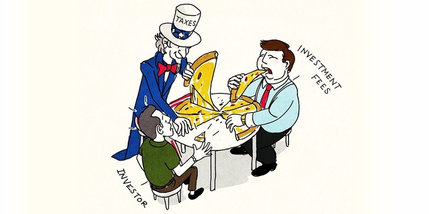
US Tax Reform Leaves Even Less of the Pie for Individual Investors in Alternatives

January 29, 2018

Tax Matters

US Tax Reform Leaves Even Less of the Pie for Individual Investors in Alternatives

By Victor Haghani and James White 1

Let me tell you how it will be
There’s one for you, nineteen for me
‘Cause I’m the taxman, yeah, I’m the taxman
Should five per cent appear too small
Be thankful I don’t take it all
‘Cause I’m the taxman, yeah I’m the taxman…

“Taxman,” by The Beatles (1966)

The Tax Cuts and Jobs Act passed into law last month will increase the wedge between pre-tax gross and after-tax net returns of many hedge funds and other private investments for high-income taxable US investors.2 Imagine a hedge fund that produces a 15% pre-fee, pre-tax return in short-term capital gains, charges the standard 20% incentive fee and 2% management fee, and also passes through 1% of miscellaneous investment expenses.3 Assume the investor lives in New York City and so pays a combined marginal tax rate of 53.5% on ordinary income.4

While the hedge fund proudly reports a salubrious 9.6% return after fees, as you can see in the table below, the investor will only be left with 2.9% after taxes. That’s an effective tax rate of 70%. Ouch!

Tag Team of Fees & Taxes Crunches Taxable Investor Returns

Pre-fee, pre-tax return 15.0%
less management fee and misc. investment expenses -3.0%
less Incentive fee: 20% of 12% -2.4%
Return after fees reported to investors 9.6%
Taxable income, after adding back in non-deductible 3% expenses 12.6%
less Taxes: 53.5% of 12.6% -6.7%
less management fee and misc. investment expenses -3.0%
After-fee, after-tax return 2.9%

What’s going on? Not only is our NYC investor paying a higher marginal tax rate than before due to the cap on deductibility of state and local taxes, but she’s also being hit by the new and total non-deductibility of management fees and investment expenses that show up in the box for “Miscellaneous Itemized Deductions” on the k-1 she receives. This is a subtle yet very significant drag on after-tax performance.5

The wedge turns into an iceberg at lower gross returns. For example, if the hedge fund had a gross return of 8.5% that would leave just 0.5% for our investor, and she’d be singing the same despondent tune as the Beatles under the 1966 Labour government’s 95% tax rate.

Meanwhile, the tax efficiency of long-term investing in the public equity market was left mostly intact by tax reform, or even slightly improved with the lower effective individual tax rate on public market pass-through vehicles, such as REITs and MLPs.6 Investors did have a momentary fright from the Senate’s “FIFO” proposal, dropped at the 11th hour, which would have taken away the benefit of choosing specific tax lots on sales.

An equity market return of just 4.5% in the form of long-term capital gains and qualified dividends would deliver the same after-tax return to our investor as the hedge fund earning 15% before fees and taxes. The wedge widens significantly further when we consider the value of tax deferral in long-term equity investing,7 and the fact that neither the IRS nor most hedge fund managers return previously paid taxes or incentive fees when you have investment losses.

Conclusion: taxable investors must expect incredible out-performance to close the after-tax return gap between high fee, tax-inefficient alternative investments and long-term investing in public market equities. While the Beatles had to leave the UK to avoid being left with one Shilling on a Pound of their income, U.S. taxable investors who want to keep a higher fraction of the gross return on their capital can achieve that goal without ever leaving home.


  1. Victor is the Founder and CIO of Elm Partners, and James is Elm’s CEO. Past returns are not indicative of future performance. This not is not an offer or solicitation to invest.
    Thank you to Larry Hilibrand for his always-helpful comments.
  2. The authors are not tax experts. This should not be construed as tax advice.
  3. This is an illustrative example. The tax characteristics of different private investment vehicles vary widely, and some may be quite tax efficient. However, what we present here is a relatively common case, and by no means the worst case.
  4. 37% Federal, 12.7% NY State & City and 3.8% Obamacare Investment Tax gets us the 53.5% top marginal tax rate for NYC residents. The rate is 40.8% for investors who live in states with no income tax.
  5. This is an even bigger issue with investments such as private equity and venture capital that charge management fees on capital committed but not drawn in the early life of their funds, resulting in a non-deductible expense that is very large as a percent of average capital invested. These deductions were excluded under the prevailing AMT rules before the recent tax changes.
  6. While the cut in the U.S. corporate tax rate from 35% to 21% was a tremendous improvement in the overall tax efficiency of stock market ownership, our analysis in this note is focused on direct taxes paid by individual high-tax-rate investors.
  7. Deferral has several potential benefits: 1) compounding at the pre-tax rate and paying tax at the end is better than compounding at the after-tax rate, 2) appreciate assets can be donated or bequeathed without paying capital gains tax, and 3) investors tend to retire to lower-tax states. See our note from November 2015 for more detail.
Read More

New Year, New CEO, New Home

January 17, 2018

In the News

New Year, New CEO, New Home

The New Year brings two exciting developments at Elm. The first is that James White, who has been working with Elm for the past year, is taking on the role of CEO. Our founder, Victor, will remain CIO and focus on devoting his time to research, writing and spending more time with investors. The second change is that James and our main office will, in the near future, be moving to Philadelphia.

Our New CEO

James studied Math at the University of Chicago, before taking a job at NationsBank’s recently acquired CRT unit (Chicago Research and Trading, a pioneer in options trading), working on their trading systems and quantitative models. He then joined Citadel in fixed income trading. In 2008, James left Citadel, and along with two partners ran a small private equity investment pool, focused mostly in Asia, and through which he held a number of executive operational roles with their portfolio companies.

James’ involvement with Elm started off with him joining our investor group about a year ago. It was through this that Victor and James started to write research notes together. In the past year, they’ve published more than a dozen on our blog as well as SSRN.com and Bloomberg. This collaboration grew into James agreeing to build an industrial-strength, state-of-the-art investment and portfolio management system for Elm, replacing our mostly spreadsheet-based systems. This Python and SQL- based system is named Ulmus (the plant-family genus for the Elm), and not only is it more scalable and secure than our previous systems, it also has significantly more functionality and allows Elm to manage our portfolios with greater cost and tax efficiency.

Hello Philadelphia

The second big development is that James and our main office will soon be in Philadelphia. Why Philadelphia? Besides cost-efficiency and proximity to NYC and our many investors in the tri-state area, it’s a great city! Check out this short clip that the city prepared to convince Amazon to choose Philly as its headquarters.

Growth in 2017

James will be a big help in managing our growth, which was significant in 2017. Our growth was thanks primarily to referrals and top-ups from our existing investors, which we very much appreciate. Investment returns of around 19% helped too. Our investor group and the assets we’re managing both grew by over 50% to over 225 investors and $600mm of assets. While the majority of our investors are finance professionals, our investor base is geographically diverse, spanning half the states in the U.S., and about a quarter comes from outside the U.S.

With best wishes for a healthy and happy 2018,

  – Victor, James and the entire Elm team

Read More

A Brainteaser Double-Feature for the Holidays

December 20, 2017

Investing 101

A Brainteaser Double-Feature for the Holidays

By Victor Haghani and James White 1

Here are two little puzzles that we discussed at an Elm dinner last week in London, at our favorite local Chinese restaurant. Our guests were sufficiently tickled that we thought we’d write them up to share with you.

Ali and Hassan: A parable from Vic’s dad

Ali and Hassan are antique dealers in the bazaar. Hassan notices a beautiful antique glass bowl in Ali’s shop, which Ali claims he was given by an itinerant dervish in return for a cup of rice. Hassan asks Ali for a price and buys the antique bowl for 10 Rials. The next day, Ali drops by on Hassan for tea and expresses regret at having sold the bowl, and buys it back for 20 Rials. Then Hassan, wishing he hadn’t let it go, buys it back for 30 the next day. This goes on day after day until 47 days later Ali visits Hassan intending to pay 500 Rials to get the bowl back. He looks high and low in Hassan’s shop, but he doesn’t see it anywhere. Hassan explains that a client came in and bought the bowl for 500 Rials. With disgust, Ali curses Hassan: “You donkey! Why did you sell our bowl – we were making such good money from it every day!”

How much money do you think Ali and Hassan individually made, or lost, from all the action? Assume Ali got the bowl for free (a bowl of rice was inexpensive back then).

How much would each of them have made, or lost, if instead of Hassan selling the bowl to a client, it had fallen off his shelf and shattered into pieces? Assume any debts between Hassan and Ali are paid in full.

Answers in footnote 2 below.2


The Two-Envelope Conundrum: Stick or Switch

We had fun playing this game for real at our dinner. We brought two envelopes, pre-stuffed with cash (Pounds, not Rials) and blank paper so the envelopes looked the same. We explained to our guests that in one envelope was a certain amount, and in the other was ten times that amount. We’d choose someone to play the game and let them select one of the envelopes and take a look inside, and then they’d be given an opportunity to stick or switch to the other envelope.

What would your strategy be? Would you always switch, or always stick, or follow some other strategy?

Before we played the game out, a quick poll suggested most were thinking their strategy would be to always switch, based on the ‘quick’ intuitive logic that a 50% chance of a 10x gain seems pretty good, regardless of the potential loss.

However, when we then played the game and the situation became concrete, it turns out our dinner guests thought about the problem quite differently. They saw the cash in the envelope our player opened (20 Pounds, in this case), and compared that to their expectation of the total value they thought we would reasonably stuff in the envelopes. Most players reasoned that we would put 100-200 Pounds in the two envelopes combined, so for an opened envelope with 20 Pounds they would switch, but if there were say 100 Pounds in the opened envelope, they would stick with it.

What this shows is that the more thoughtful line of analysis uses the fact that in practice we will have some prior expectation regarding the distribution of the value of the game – that is, how much money might be in the two envelopes combined. In this case, a profitable strategy does exist, which is to switch only if the money found in the first envelope is low enough relative to our prior expectation.3 And, as always, the investor’s individual risk aversion comes into play in that switching also has to be attractive enough to compensate for the risk involved. Conversation around the table went quickly from these two brainteasers to a puzzle on the minds of many: Bitcoin, crypto-currencies, and the fascinating problem of putting a value on them.4 The two envelope problem seemed to be relevant to how some of our party were thinking about Bitcoin, in that their plan was to hold on until the chance of another big upward multiple was unlikely.

Even if you don’t find either of these two puzzles of relevance to your future investing, we hope they give you and your family some fun around the table this holiday season.


  1. Victor is the Founder and CIO of Elm Partners, and James is Elm’s CEO. Past returns are not indicative of future performance. This not is not an offer or solicitation to invest.
     

    Thanks to Vic’s dad for the Ali and Hassan parable and to Jeff Rosenbluth for his guidance on the two-envelope problem, which he used as an illustration while teaching at the NYU Courant Institute of Mathematical Sciences.

  2. The answer to the first question is that together they made 500 Rials, 250 Rials each. Perhaps easiest to see if you think about Hassan selling it for 20 Rials after the first exchange, and then both of them would have made 10 Rials of profit from it. The answer to the second question is that when the dust, and payments between them, settled, Ali would have made 250 Rials and Hassan would have lost 250 Rials.
  3. We encourage you to read this Wiki entry which provides an excellent treatment. Another path to greater intuition about the problem is to set up a Monte Carlo simulation of the game.
  4. Some, like Professor Aswath Damodaran of NYU’s Stern School, argue that Bitcoin can be priced but not valued (here).
Read More

Discussions on Risk Parity and the Sharpe Ratio

December 11, 2017

Tax Matters

Discussions on Risk Parity and the Sharpe Ratio

In our ongoing writing on the topic of investment sizing and portfolio choice, we recently published two articles that discuss the use of Sharpe Ratio in building portfolios with the highest expected risk-adjusted return. In the first note, Some Clarity on Risk Parity (Bloomberg Prophets), we showed how a levered Risk Parity portfolio and a Traditional unlevered equity/fixed income balanced portfolio could both be derived from the same basic expected utility maximization toolkit. We went on to show that a relatively small difference in investor risk and leverage preferences would tip the investor to preferring one versus the other type of portfolio.

In our second note, A Brief History of Sharpe Ratio and Beyond, we dug deeper into the question of how much investors can rely on maximizing the Sharpe Ratio in choosing the investment portfolio best for them. As we discussed in our first note on Risk Parity, we explain why Sharpe Ratio isn’t enough for investors who have an aversion to leverage. We show why, and to what extent, investors should be willing to trade off a lower Sharpe Ratio versus a higher expected return on their portfolio.

Read More

A Brief History of Sharpe Ratio, and Beyond

November 26, 2017

Investing 101

A Brief History of Sharpe Ratio, and Beyond

By James White and Victor Haghani 1

Early in the 1950s, academics and investors started proposing in earnest a variety of summary statistics to capture in a single number the quality of an investment. It was recognized that expected return wasn’t quite enough, because two investments with the same expected return could have dramatically different levels of risk. Pretty much everyone agreed that the quality statistic should be something like “expected return/risk”, but the devil was in the details, and especially in the definition of risk. In the 1960s, William Sharpe was a graduate student working with Harry Markowitz on Modern Portfolio Theory and the Capital Asset Pricing Model, work for which they’d later share a Nobel Prize along with Merton Miller. In 1966 Sharpe proposed a risk/reward ratio which he called the “reward-to-variability ratio,” or “R/V Ratio” 2 defined as:

Expected Return – Risk Free Rate Standard Deviation of Return

The name didn’t quite stick. Thirty years later, in a paper cheekily titled “The Sharpe Ratio”, 3 Sharpe himself concedes that his original term, which doesn’t exactly roll off the tongue, never gained popularity. Once he himself suggested referring to the measure as the “Sharpe Ratio,” the term as we know it today fell into common usage.

Though the original name wasn’t a hit, the concept was: a measure originally coined in the very specific context of a theoretical model came to be the de-facto standard amongst academics and investors for measuring the risk/reward quality of a wide variety of real-world investments.

Today use of Sharpe Ratio in both language and practice is ubiquitous, and naturally critiques of its use are nearly as ubiquitous. Some of the core critiques are:

  • If Risk is taken to mean Risk of Loss, Standard Deviation and Risk are synonymous only when returns are Normally distributed. Many investments, such as corporate bonds, have asymmetric or fat-tailed return profiles, causing Sharpe Ratio to significantly mis-state the true riskiness of the investment.4
  • Limited historical data can result in a Sharpe Ratio estimate which is significantly biased.5

Here we’d like to focus on a separate issue which arose from our note “Some Clarity on Risk Parity.” In that note, we said that if unlimited leverage is available to the investor at the risk-free rate, then the optimal portfolio from a risk-adjusted return standpoint will be the one with the best Sharpe Ratio, levered to give the optimal amount of expected return appropriate to the investor’s degree of risk-aversion. For many investors though, unlimited leverage on good terms isn’t feasible,6 either because the cost is higher than the risk-free rate, or because the investor just wants to avoid leverage.7

For the leverage-constrained investor, is Sharpe Ratio still all we need to look at to determine the best portfolio? As you’ve probably guessed, the answer is no: in the presence of leverage constraints, both Sharpe Ratio and the level of expected return are material factors in determining the portfolio with the best risk-adjusted return. In the chart below, we illustrate this in a simple two-asset case, showing the Sharpe Ratio and Risk-Adjusted Return from each possible combination of stocks and bonds, assuming the investor has a “typical” degree of risk aversion8 and her wealth is fully invested:9

We can see that the portfolio with the best Sharpe Ratio is about 20%/80% Stocks/Bonds, but the portfolio with the best risk-adjusted return10 is about 45%/55% Stocks/Bonds.11 We believe allocating assets proportionally to risk-adjusted return is sound investing practice, and in the case of assets which follow a random-walk,12 risk-adjusted return is fortunately easy to calculate:

Risk-Adjusted Return = Expected Return – 1 2 γσ2

where γ is the investor’s level of risk-aversion and σ the asset’s volatility.

This relationship also gives us a formula for the trade-off between Sharpe Ratio and level of return given a leverage constraint. Consider our 45%/55% optimal un-levered portfolio from above – if instead of investing in this portfolio we were able to earn a higher expected return, but with a lower Sharpe Ratio, how much lower Sharpe Ratio could we bear and still be no worse off in terms of risk-adjusted return? The answer is:

  SR* = R √ γ 2δ + γσ2

where SR* is the Sharpe Ratio which gives a fully-invested portfolio having return R* = R + δ the same risk-adjusted return as a portfolio with expected return R and volatility σ.

For a brief thought experiment, consider an asset with expected excess return of 4% and risk of 4% , for a (very good) Sharpe Ratio of 1. The risk-adjusted return of this asset is 3.78%13, and optimally, our portfolio allocation would greatly exceed 1, i.e. we’d optimally be highly levered. However, we have a leverage constraint, so instead we just hold our entire portfolio in this asset. Now we’re given the chance to switch into an alternative asset with a somewhat higher expected return of 4.5% – how much lower a Sharpe Ratio would we tolerate to still make the switch? The result is pretty surprising:

Here we have a list of hypothetical assets, all of which have the same risk-adjusted return, and we can clearly see the Expected Return/Sharpe Ratio trade-off at work – we’d switch to being fully invested in the 4.5% asset if its Sharpe Ratio is better than 0.62, a material discount from the reference portfolio Sharpe Ratio of 1.

Conclusion

As we can see from our thought experiment, in the presence of leverage constraints two portfolios with dramatically different Sharpe Ratios can be equally desirable. In the case of our stylized stock/bond example, the difference between the highest-Sharpe portfolio and the optimal portfolio is material but not too extreme – only about 0.25% per annum in risk-adjusted return. But this difference can be much bigger depending on your assumptions, especially if some of the assets involved have levered, asymmetric, or structured payouts. Our general point is that for most investors, and especially those with a desire to limit leverage, Sharpe Ratio is a useful and important metric, but doesn’t deliver the full-credit answer. To achieve the best expected risk-adjusted returns, investors with capital or leverage constraints need to think a step further, taking both Sharpe Ratio and the absolute level of their investments’ excess return into the mix.14


  1. This not is not an offer or solicitation to invest, nor should this be construed in any way as tax advice. Past returns are not indicative of future performance.
  2. Sharpe, William F. “Mutual Fund Performance”. Journal of Business, January 1966, pp. 119-138. (p. 123 in particular)
  3. William F. Sharpe, “The Sharpe Ratio”, Journal of Portfolio Management, 1994.
  4. Even relatively “vanilla” markets, such as the Broad US Equity market, can display markedly non-Normal behavior, especially over short to medium time-periods. Over longer time-periods this non-Normal behavior tends to lessen, though there’s still disagreement over whether Normal distributions are a sufficiently good model for long-term returns.
  5. Due to sampling error, survivorship bias and the critique above.
  6. Or accessing such leverage requires investing through 3rd-party managers with their own fee structures and potential agency issues.
  7. Consistent with a focus on capital preservation.
  8. We’ll define “typical” here as that degree of risk aversion that would maximize expected utility by investing 100% of savings in a stock/bond portfolio with a 60/40 mix. With our example numbers, this implies a coefficient of risk aversion in the Merton model of ~3 (2.7 is what we use in numerical examples throughout). For readers familiar with the Kelly Criterion, this means our investor is ~3x as risk averse as a Kelly bettor.
  9. We’re making a material assumption here that, in the absence of leverage, the investor optimally wants to be fully invested, vs. keeping part of her wealth in cash. That’s definitely not true in general, but in the case of our specific 2-asset example here, it is in fact true.
  10. In this context used interchangeably with “Expected Utility.”
  11. We assume that stocks and bonds can be described by un-correlated geometric Brownian motions, with stocks having 4% expected excess return and 16% volatility, and bonds having 1% expected excess return and 4% volatility.
  12. And investors with Constant-Relative-Risk-Aversion (CRRA) utility.
  13. Using the same risk-aversion as above.
  14. Your authors like the expected-utility framework for unifying these considerations within a single user-friendly toolkit, but we feel the specific method is less important than the general idea of translating expected returns into risk-adjusted returns before making your investment decisions.
Read More

HHHHHHHHHHHH: Is there a message in there?

November 20, 2017

How Elm Works

HHHHHHHHHHHH: Is there a message in there?

By Victor Haghani and James White 1

The 12-month winning streak of the stock market through the end of October reminded me of a Friday afternoon on the Salomon trading floor in early January 1987.2 The markets had closed, the day’s trades were confirmed and we were sitting around discussing weekend plans. In walked six and a half feet of the most enthusiastic and well-liked of all the Salomon MDs, a man who believed nothing was impossible.3

“How about that stock market! Up every day this year so far – six days in a row! I think it’s going to be up every day this year. What odds would you guys give me on $1,000 that I’m right?”

We perked up. There were another 245 trading days left in the year, and even if we assigned an 80% chance to the market being up each day, the probability that it would be up the next 245 in a row was about a trillion trillion to one.4

We agreed to syndicate the risk among five of us, and we offered him odds at 5,000:1, but only on $50. He scoffed and walked away dissatisfied – no bet.5 Then, as if to show us that anything remotely possible might just happen, we watched the Dow go up every day for the next seven days, an 11% rally altogether, until the streak finally ended on the 14th day.6

Bloomberg just published a short note we wrote (here) that takes a more in-depth look at stock market streaks. We reviewed 150 years of US stock market history and found that there have been six streaks of 12 months or longer. While it’s very likely we would witness one streak of 12 or more winning months in a row, it is highly unlikely to see six or more such streaks if the stock market followed a random walk, with each month’s return independent of prior returns.

What history suggests is that, in the short to medium term, the stock market exhibits momentum, or trending, which likely goes hand-in-hand with longer term mean reversion.7 As you know, at Elm we believe it makes sense to take account of valuation and momentum in the asset allocation decision. While the past is not necessarily indicative of the future, our review of stock market streaks does not contradict our view of market behavior.


  1. Victor is the Founder and CIO of Elm Partners, and James is Elm’s CEO. Past returns are not indicative of future performance. This not is not an offer or solicitation to invest.
  2. My memory of these events is a bit fuzzy, but the main aspects of the story are accurate.
  3. For those readers who were at SB at the time: OG.
  4. And it took a good few seconds for our HP12C to do that calculation.
  5. We didn’t think about it in these terms at the time, but it turns out that this was a positive expected utility bet for us, even assuming the chance of us losing was 0.01%, rather than 2.0e-24.
  6. Even more unlikely than the stock market’s 13-day winning streak at the start of 1987 was the Monday later that same year, on October 19th, when the stock market fell by over 20% in one day.
  7. You may be wondering what happened after each of the five market winning streaks of 12 months or more ended. The average total return following each of those five streaks, starting one month after the streak ended, was about 15%. It was positive in four out of five of those cases. While five data points do not produce a result of statistical significance, this result is not inconsistent with the hypothesis that the stock market displayed positive momentum or trending in the past.
Read More