Elm Wealth Research

It seems just about everyone I talk to these days is underwhelmed by the long-term expected return of the global stock market. I too am more worried than normal about owning equities. However, my defensiveness arises from their negative momentum, not their valuation, which I see as surprisingly attractive.

The valuation picture is blurred by the dramatic divergence between US and non-US equities. For the past four and half years, the US equity market has outpaced non-US equities by more than 10% a year. After that relative outperformance, US equities do appear overvalued, but the attractive valuation of non-US markets more than compensates in a global portfolio.

The table below shows the cyclically adjusted earnings yields (using the past 10 years of earnings) of each regional equity market. The Baseline regional weights I’m using fall in between the weights published by MSCI and those calculated by Bloomberg using their WCAP function.¹

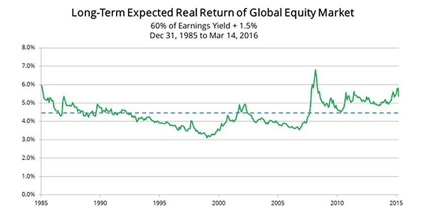
The earnings yield of the global equity market is 6.6%. To get to an estimate of the long-term expected real return, I assume that 60% of earnings can be paid out in dividends (besides sounding like a reasonable assumption, it also happens to be the average payout ratio from 1915 to 2015 in the US), which will grow at about 1.5% above inflation in the long term. Many observers prefer the even simpler estimate of just using the earnings yield itself, which is 6.6%, but I prefer basing the estimate on cash flow to investors, which is generally more conservative.

This results in 5.5% for the long-term expected real return for global equities (6.6% * 0.6 + 1.5% ).²

So how attractive is a 5.5% expected return above inflation? Here are four perspectives to consider:

• US equities returned 5.4% after inflation in the 50 years from 1965 to 2015, which many people view as having been a good time to be an equity investor (although not nearly as good as the 8.2% from 1915 to 1965).
• The chart at the top shows that 5.5% is well above the average expected return of 4.5%. It is in the top decile of expected returns calculated this way since 1985, a period of time longer than the careers of 80% of the people currently employed in the finance industry.³ We expect the average expected return prior to 1985 would be higher, but we don’t have readily available non-US data to extend the chart further into the past.
• By contrast, other assets, such as fixed income and real estate, are currently offering low expected real returns, in the bottom decile of expected returns over the past 30 years. It is difficult to come up with a simple prospective measure of expected real returns for alternatives such as hedge funds, but they certainly have been struggling recently to generate the attractive returns they produced in the 80s and 90s.
• Caution: equities can get a lot cheaper, quickly. Just a month ago, global equities were more than 10% lower than they are now, in case we need any reminder. While 5.5% appears attractive as a long term expected real return, we need to keep in mind that we may see much higher expected returns than that in the future.

Bottom line:

Global equities are pretty attractively valued, and when they enter a period of positive momentum, we’ll probably see very healthy returns.

---

1. MSCI bases its weights on strict investible market cap data, while Bloomberg bases theirs on unrestricted market cap. The Baseline weights used here go beyond market cap, using other economically relevant data to compute weights. See this note for details, and here for a further comparison of weighting schemes.
   
2. Based on the belief that earnings and dividends will grow at less than the rate of real GDP growth due to various slippages. For a more detailed discussion, watch this video, and read this short note. Furthermore, if we think of this as the central case in the return distribution, and if we believe the long-term return is distributed relative symmetrically around this value, then there is a convexity adjustment that makes investing in equities even more attractive.
    

   A back-of-the-envelope illustration is to note that if we thought there were two equally likely long term (say 30-year) outcomes for the real return, of say, 5.5% + 2% and 5.5% – 2% , we would see that the return associated with the expected value of equities would be 6.02%, or 0.52% higher than the 5.5% base case.
   

3. From US BLS data, here.
   

By Victor Haghani and Samantha McBride ¹

Introduction

A thriving investment manager started his presentation to a roomful of potential investors, saying:

“Before I tell you what I do, I’m going to ask and answer the most important question you should put to me: Who is losing the money that I’m going to make for you?”

“The answer: return chasers.”

---

At first, this sounds reasonable, at least with regard to investment returns which are not explained by risk. But then, on further reflection, one has to ask: What about trend following, arguably the best systematic investment strategy of all time? Why was he silent on what many consider the “premier anomaly?” ² More troubling still, how can trend following have worked so well, while “return chasing,” which sounds like the same thing, be so misguided as to be the primary source of the superior returns of smart investors?

What follows is an attempt to answer that question, which may be useful both in making sense of history and thinking about the future.

Definitions of Trend-Following and Return Chasing

Fortunately, half of the problem is straightforward; trend following is pretty well-defined. Set in the context of an investor who wants to hold a baseline allocation in equities of 50%, with the other 50% in cash, a simple trend following investment strategy would be:

Trend Following: If the past one year ³ stock market return was good, say prices have gone up by more than 2.5% after inflation, hold 100% in stocks; if it was wasn’t good, hold 0% in stocks.

It’s hard to come up with a simpler strategy. And what is truly remarkable is that it’s hard to come up with one that has done better. For example, from 1975 to present, it added about 2% a year to the returns of a balanced long-only portfolio of 50% US equities and 50% T-bills, while significantly reducing risk.⁴ And this simple investment rule has been shown to have worked virtually everywhere and every when.⁵

So that’s trend following. Unfortunately, “return chasing” doesn’t have an agreed-upon definition.

While trend followers proactively follow a pre-defined set of rules, which are well-documented in the academic literature, return chasers act in a more discretionary and reactive way. Return chasers are often unaware of their behavior, creating a slower-moving, self-reinforcing herding phenomenon, based on the simple, readily available and intuitively appealing heuristic of recent past returns.

This description suggests the following definition:

Return Chasing: When the past one-year return has been good, buy some stocks, and when it’s been bad, sell some.

The key difference with trend following is that return-chasing behavior is a flow, which continues as long as returns are either good or bad, while trend followers buy as soon as the return has been good and hold until the return becomes bad, and then they sell, and don’t do anything until the return has been good again, and then they buy and hold again, etc.

Below is a chart that compares the positioning of a return chaser and of a trend follower in the case of a very stylized cyclical asset price path with a nine year cycle. The line of the asset price is green when the last one year return is positive and red when it’s negative. If you look carefully, you can see that the sign switch (the color change) occurs shortly after the market peak or trough. Notice how the trend follower changes his allocation abruptly, capturing most of the moves up and down in the asset price, while the return chaser is slow to adjust his holdings, which results in him losing money from his dynamic positioning, as he winds up with his maximum long holding just after the market peak and his minimum holding just after the market hits bottom.

The next big question we need to ask is, do the return chasers lose money in more realistic scenarios other than this highly stylized case above? There are at least two places we can look for an answer: 1) check if they’d have lost money applying that rule historically, and 2) using a Monte Carlo simulation to see how the strategy would perform over many plausible histories.

Historical Analysis

Let’s start with a historical look at US equities. We used Professor Robert Shiller’s monthly US equity data from his website, which goes back to 1871. We compared three strategies: 1) static 50/50 Equity / T-bill portfolio, rebalanced monthly, 2) the momentum strategy as described above, and 3) a return-chasing strategy, wherein the investor increases or decreases his exposure to stocks each month by 20% of however much the past year’s real price return was in excess of 2.5%.⁶

The table below shows this didn’t work out very well for the return chaser, underperforming the static weight buy-and-hold investor by over 1% a year. You may be even more surprised to see how well the simple momentum strategy did, outperforming the static weight buy and hold by 2% to 3.5% a year, even though superficially it seems so similar to the return chaser. Of course, we shouldn’t expect all return chasers to be using a one-year look-back in deciding their asset allocation, but it turns out they would have also done poorly using a broad range of other look-back windows: six months and two, three, four and five years as both straight look-backs and as moving average windows. We found the same order of magnitude results in the case of the MSCI World developed index from 1975 to the present.

	50% Equity 50% T-bills	Return Chaser	Momentum Investor
Real Return
1872 – 2015	4.86%	3.70%	8.42%
1925 – 2015	4.46%	3.11%	7.59%
1975 – 2015	5.77%	4.67%	7.71%
vs. 50% Equity 50% T-bills
1872 – 2015		-1.16%	3.56%
1925 – 2015		-1.35%	3.13%
1975 – 2015		-1.10%	1.94%

The chart below shows the return chaser’s asset allocation (the blue bars) over the whole time period, with the stock market real price performance in the orange line, off the right hand scale, in log space. The return chaser’s asset allocation chases the market, and, significantly, it tends to have its biggest exposure shortly after the top of the market and its lowest exposure shortly after the bottom.

By contrast, the momentum strategy jumps up to being over-allocated more quickly than the return chasing approach, and also gets under-allocated more quickly. One description would be that trend followers “front-run” the slower adjustment of the return chasers, giving the trend an initial boost. Ironically, the return chasers probably feel they are being prudent and wise to adjust their allocations slowly, scaling in and out of their investments as they get confirmation they’re doing the right thing, as compared to trend followers who dive in fully to their adjustments and hold until it’s time to go the other way. The trend followers are more frenetic in their activity; as configured, they have ten times higher turnover than the return chasing strategy.

The Not-So-Curious Case of Investor Returns Being Substantially Lower Than Fund Returns

Supportive, but indirect, evidence for the notion that return chasers are losing money is the finding that mutual fund investors have earned 1.5% to 3% a year lower returns than the returns of the funds they invested in.⁷ This is separate from the effect of fees on investor returns, which gets so much coverage in the financial press; rather, it has to do with the timing of investor flows. The effect probably comes from a combination of poor market timing and poor dynamic selection of funds themselves, putting money into funds that are hot and redeeming from those that are not. That dollar-weighted investor returns have been lower than fund returns historically has not attracted as much attention perhaps because it’s a story wherein the perpetrator and the victim are the same party: the investor.⁸

Monte Carlo Simulation

Let’s now turn to exploring the question through Monte Carlo simulation. We’ll assume two assets: a risky one (think equities) and a zero risk one (cash). We generate series of prices for the risky asset by starting at a price of 1, and we model the price dynamics as having three components: 1) a random weekly shock, which is normally distributed with mean of 0, and an annual standard deviation of 16%, 2) mean reversion, where the price moves back to 1 at a rate of 25% a year (or roughly 0.5% of the way each week), and 3) a price impact of the return chasers, where for every 1% change in their desired allocation to equities they move the price up or down by 0.5%. This price impact is consistent with what would need to happen to equity prices if roughly 12% of the stock market were held by return chasers who started with a 50/50 allocation between equities and cash and wanted to move to 51/49 and the other holders of equities didn’t want to sell to them.⁹ And, as with our historical analysis, we assume they will change their allocation each month by 20% (about 5% each week) of whatever the past one year excess return has been, with a cap of 100% and a floor of 0%. We assume no price impacts from other market participants, such as trend followers or value investors, which is a critical assumption the relaxation of which is discussed later.

In the simulation approach we again looked at three investment strategies: 1) a static 50/50 equity/cash monthly rebalanced portfolio, 2) return chaser who starts out 50/50 and 3) a trend follower who is 100% invested in either equities or cash. We assume 0 transactions costs in all these strategies. The table below shows the results for 5,000 paths of 20 year investment periods based on weekly simulated prices.

	Return Chaser	Momentum Investor
vs. 50% Equity / 50% Cash	-2.0%	7.3%
Sharpe Ratio	-0.18%	0.62%

As you can see, the return chasers lose money compared to the buy and hold investor, and the trend following investors make money. Interestingly, the return chaser shortfall is not too far from what we see empirically in the studies comparing dollar-weighted investor returns and fund returns. Also, it is noteworthy that the Sharpe Ratio of the return chaser at -0.18 is close enough to 0 that it would take a long time to conclude that he is following a harmful strategy. The momentum investor, on the other hand, generates a high enough Sharpe Ratio to gain confidence within say a 10-year horizon that his positive results were not just a random outcome. These results are robust to the following range of parameterizations: we doubled and halved each of the parameters describing the impact of return chasers and the coefficient of mean reversion separately and jointly, and the same pattern and order of magnitude of results held in all eight perturbed cases.¹⁰

Return Chasing: A Simple but Expensive Heuristic

Of course, this is just a guess at the nature and prevalence of return chasing strategies. It’s very difficult to figure out how many return chasers there are, as many return chasers are not even aware that they are behaving that way. In fact, we suspect there are return chasers reading this note thinking: “What a silly way to invest. There can’t be many people who do this.” Investing is a complex affair, and when faced with complexity, we rely on simple heuristics. There is no heuristic simpler or more to hand than looking at past returns. Of course, that means ignoring the most common disclaimer in investing, “past results are not necessarily indicative of future returns,” but as the saying goes, “let’s not allow facts stand in the way of a good story.”¹¹ Even if individual investors do not move gradually in their investments, as a group they may behave that way, as herding and network effects result in some investors being the leaders (the trend followers) and others moving more slowly and hence doing worse than the average of the return chasers.

Gradualism seems like a good way to deal with uncertainty, and it reduces transactions costs, and possibly regret too. Unfortunately, what seems like a sensible approach turns out to be a very expensive one.

Explanation for Momentum

An understanding of why a strategy has worked in the past is essential in deciding whether to stick with it in times when it’s not profitable. This simple model of return chasers adds to other plausible explanations for why trend following based on momentum in asset prices in the roughly one year horizon has been so profitable and ubiquitous.¹² Barberis and Shleifer (2003) and Vayanos and Woolley (2013) provide comprehensive and rich treatments of this phenomenon, relating return chasing behavior to investors using past absolute and relative returns as primary indicators of manager competence or expected future relative returns across investment styles or asset classes. Models grounded in return chasing behavior complement other popular rationales for momentum in asset prices such as anchoring (under-reaction) and herding (over-reaction).

Another suggestion for a definition of return chasing is that it is the pursuit of trend following rules with too long of a horizon. While this may explain how prices move away from fair value and create opportunities to benefit from long term mean reversion in asset prices, it has two shortcomings in accounting for momentum. First, we need to show that it loses money, but in fact, trend-following in US equities using a two-, three- or four-year window actually made money historically, and it is somewhat unlikely that return chasers focus almost exclusively on five-year and longer returns in driving their return chasing.¹³ Second, unlike return chasing as defined herein, it is hard to see how trend following strategies with too long a window generate price impact patterns that would make trend following with a one-year window profitable. A more exhaustive review of other possible definitions of return chasing would be valuable.

Explaining Other Profitable Active Strategies

The impact of return chasers explains strategies beyond simple trend following. Naturally, it explains all the strategies that are (sometimes unrecognized) cousins of trend following such as those using tight stop losses to “cut your losses early and let your profits run” (PT Jones, Soros, L Bacon, BH), or the value investors who intentionally adjust their allocations slowly through “sliced” or “lagged” strategies (GMO), or those who unintentionally move slowly because they invest in illiquid investments that take time to analyze (Oak Tree). This simple model also helps us understand a possible source of return for pure value investors, as, about half the time, return chasers move prices away from fair value. The model also provides some testable predictions, such as that we should observe reversion to fair value being a faster moving adjustment than the move away from fair value. While value investing has a long tradition with persuasive proponents on its side (from Graham to Buffett to Klarman), it does not appear to generate as attractive a return profile as trend following, which perhaps is what we should expect from a strategy that has so much intuitive appeal as value investing.

Looking Forward

In conclusion, that thriving investment manager was on to something: despite its superficial similarity with the historically profitable strategy of trend following, return chasing may indeed be investing’s “original sin.” Worse, when the return chasing crowd becomes too big, they may be the primary cause of the too frequent bubbles and busts our system suffers. From the narrower perspective of trend followers and value investors, return chasers may be the ones paying the rent, although every once in a while they thin out the ranks of value investors too. What the future holds is not so clear. It depends on the relative size of capital engaged in return chasing, trend following, value investing and other dynamic investment strategies. The attractive historical returns of trend following and value investing will likely continue to attract capital to those strategies, while the ongoing education and “passive-ication” of investors ought to reduce return chasing. Capital dedicated to trend following will continue to be volatile. In most investment strategies it is possible to identify the source of the expected return, by for example measuring the relative PE of value stocks as compared to growth stocks. For investors considering trend following strategies the main way to calculate expected returns is, ironically, with reference to historical returns. Trend following produces a Sharpe Ratio in the vicinity of 0.5, which may not be high enough (especially when high fees are involved in delivering it) to hold dedicated capital in the long term. Just how far these relative changes in investor behavior go is hard or maybe impossible to predict as the complex and adaptive interaction between the strategies, including return chasing of the strategies themselves, may mean a long-term equilibrium just does not exist.

---

Further Reading and References:

• Asness, Clifford S., Tobias J. Moskowitz and Lasse Pedersen. “Value and Momentum Everywhere,” Journal of Finance. (2013)
• Barber, Odean. “The Behavior of Individual Investors.” Working Paper. (2011)
• Barber, Odean. “Trading Is Hazardous to Your Wealth: The Common Stock Investment Performance of Individual Investors,” Journal of Finance. (2000)
• Barberis, Shleifer. “Style Investing,” Journal of Financial Economics. (2003)
• Borri, Cagnazzo. “Chasing Stock Market Returns.” Working Paper. (2015)
• Chabot, Ghysels and Jagannathan. “Momentum Trading, Return Chasing, and Predictable Crashes.” Working Paper. (2014)
• Cochrane, John. “The Dog That Did Not Bark: A Defense of Return Predictability,” Review of Financial Studies 21(4) 1533-1575. (2008)
• Dichev, Ilia. “What are stock investors actual historical returns? Evidence from dollarweighted returns.” Working Paper. (2014)
• Fama, Eugene F. and Kenneth R. French. “Dissecting Anomalies,” Journal of Finance 63:1653-1678. (2008)
• Friesen, Sapp. “Mutual fund flows and investor returns: An empirical examination of fund investor timing ability,” CBA Faculty Publications. (2007)
• Geczu, Samonov. “215 Years of Global Multi-Asset Momentum: 1800-2014.” Working Paper. (2015)
• Gnedenko, Boris and Igor Yelnik. “Dynamic Risk Allocation with Carry, Value and Momentum.” Working Paper. (2014)
• Grimaldi, Marianna and Paul De Grauwe. “Bubbling and Crashing Exchange Rates,” CESifo Working Paper Series No. 1045. (September 2003)
• Hilibrand, Lawrence. “Expected Returns, Over-Extrapolation and Asset Pricing.” Working Paper. (2015)
• Hurst, Brian, Yao Hua Ooi, Lasse Pedersen. “A Century of Evidence on Trend Following Investing.” Working Paper 24. (2012)
• Jegadeesh, Narasimhan and Sheridan Titman. “Returns to Buying Winners and Selling Losers: Implications for Stock Market Eciency,” The Journal of Finance, vol. 48, no. 1, pp. 65-91. (1993)
• Kahneman, Daniel and Amos Tversky. “Judgment Under Uncertainty: Heuristics and Biases,” Science. (1974)
• Kinnell, Russell. “Mind the Gap 2015,” Morningstar. (2015)
• Lou, Dong. “A Flow-Based Explanation for Return Predictability.” Working Paper. (2012)
• Maymin, Fisher. “Past performance is indicative of future beliefs,” Risk and Decision Analysis. (2010/11)
• Moskowitz, Ooi and Pedersen. “Time Series Momentum,” The Journal of Financial Economics vol. 104. (2012)
• Pirrong, Craig. “Momentum in Futures Markets.” Working Paper. (2005)
• Vayanos, Woolley. “An Institutional Theory of Momentum and Reversal,” Review of Financial Studies. (2013)

---

1. This not is not an offer or solicitation to invest, nor should this be construed in any way as tax advice. Past returns are not indicative of future performance.
   The authors would like to thank Larry Hilibrand, Richard Dewey, Paul De Grauwe, Andy Morton, Bob Shiller, Antti Ilmanen, Ayman Hindy, Aneet Chachra, David Modest, Phil Maymin and Jeff Rosenbluth for their contributions to this research. We thank Bob Shiller for his generous provision of the data that makes research like this possible.
   
2. These are the words of Gene Fama and Ken French (2008). This note is primarily concerned with what in the literature is referred to as time series momentum, as opposed to cross-sectional momentum, however, most of the modeling and discussion can be applied to both manifestations of asset price momentum.
   
3. We could have used 6 or 18 months, or the average of the past year for the look-back window, and all these as well as many other variations would all have been similarly effective.
   
4. See “Investing for the Rest of Us,” Haghani and Dewey (2011).
   
5. See, for instance, this paper: “Time Series Momentum” (2010).
   
6. We limit the investor’s equity exposure to be greater than 0% (i.e. no shorting) and less than 100% (no leverage).
   
7. Let’s illustrate with an example. Suppose we look at $1 invested in some mutual fund over a ten year period, with all dividends reinvested. Let’s say that $1 grew into $2.16 after 10 years. We’d say the fund had an 8% return (1.08¹⁰ = 2.16). That’s what’s called the “fund return.”
   Now let’s take a simple case where the fund started out with $100mm of investor assets, and for five years grew those assets at 12% a year, to $176mm. At that moment, new and/or existing investors invest a further $200mm into the fund, bringing its assets up to $376mm. Now for the next five years, the fund grows at only 4.14%, which I chose because growing for five years at 12% and then five more years at 4.14% gives an 8% return over the whole period. At 4.14%, the $376mm grows to $460mm at the end of 10 years, giving an investor dollar weighted return of 6.44%, a whole 1.56% lower than the fund return.
   
8. See these sources to go deeper: Morningstar’s “Mind the Gap,” Dichev, Barber & O’Dean, Friesen & Sapp, or Dalbar.
   
9. Larry Hilibrand pointed out to us the following calculation: Imagine that investors in aggregate have 50% of their savings in equities and 50% in cash. If all investors want to increase their equity holdings to 51%, the only way that can happen (assuming companies don’t issue more equity) is for the price of equities to go up so everyone’s equity holdings on average are 51%. For an investor with a portfolio of $100, that means that the $50 they have in cash needs to become 49% of their portfolio, and hence their total portfolio needs to be worth $50 / .49 = $102.04 , and so their $50 equity holdings has to go up in price by $2.04, or 4.08%.
   So a 1% increase in allocation would lead to a rather large 4% move in equity prices. Hence, expecting that if return chasers increased their equity holdings by 1% we’d see a price impact of 0.5% is quite a conservative assumption in terms of how small a part of the overall market return chasers would need to comprise, or how big the value investors are, who will tend to decrease their holdings when prices are pushed up by return chasers. Starting at allocations other than 50/50 give higher sensitivities. For example, a 1% increase in equity allocation from 25% or 75% would require a 5.4% increase in equity prices. In general, dP / dS = 1 / (S * (1 – S)), where S is the starting allocation and P is the equity market price.
   
10. Removing the (0,2x) bound on how far return chasers can move from their baseline exposure can lead to runaway asset prices, which results in unrealistically high returns for return chasers and trend followers, and the extinction of value investors.
    
11. Return chasing doesn’t have to be a “mistake.” It can also arise from other pro-cyclical phenomena, such as employee bonus payments being positively correlated with a booming stock market and being invested upon receipt (e.g. Bernanke et al’s Credit Channel/Financial Accelerator theories).
    
12. See Moskowitz, Ooi and Pedersen, “Time Series Momentum” (2012), Asness, Moskowitz and Pedersen, “Value and Momentum Everywhere” (2013), or Haghani and Dewey “Investing for the Rest of Us.”
    
13. A six-month momentum window is also profitable, so the too short a window explanation doesn’t fit either.
    

We’re often asked about Elm Partners’ US office in Jackson Hole, Wyoming. Below is a short video shot by my son Josh using his quadcopter a few days ago, all within a few miles of JHHQ. Music by Adam.

What better answer is there to: “Why Wyoming?” Enjoy, and come out for a visit.

Best wishes for the New Year,
  – Victor

Victor sat down with Chris Riback of Working Capital Review to discuss his career, his thoughts on investing, and how Elm came to be.

Read the full article here.

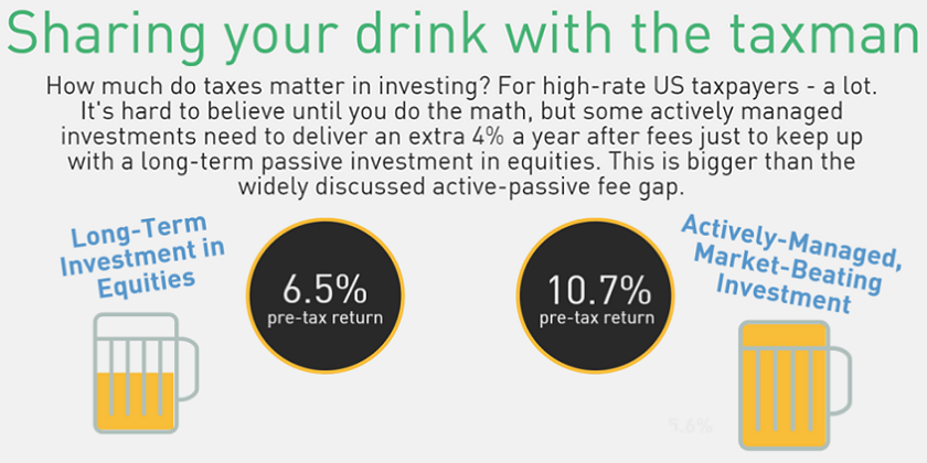
The passive vs active investing debate usually centers on low vs high fees and the plausibility of superior investment performance. For many taxable investors, taxes can matter more than either of those, as there can be a huge difference in the slice of returns you pay in taxes between passive and active investment styles. We put together an infographic to illustrate this difference in a practical example for a US high rate taxpayer.

Assumptions and discussion of other cases:

Tax is a complex topic.¹ Each of us has a different tax situation, and even within a family, different pools of savings are taxed differently. I based this note on the case of a high income US taxable investor, resident in a no-income-tax state (e.g. Texas, Florida, Wyoming). I assume (perhaps optimistically) today’s tax rates, and tax rules, stay constant in the future. Today’s federal tax rates are 39.6% for short-term capital gains and ordinary income, and 20% for long-term capital gains and Qualified Dividends. All investment income is subject to the 3.8% Affordable Health Care tax (aka Obama-care tax).² There are a variety of limitations on deduction of investment related expenses in the tax code, which can make a big difference in after-tax returns. In the base case, I have assumed miscellaneous itemized deductions are only partially disallowed, but I also present the case of full non-deductibility of these expenses.

I’m comparing two fairly extreme cases, but they are not the most extreme I could have chosen. For example, for tax-payers subject to high state taxes the gap would be even greater.

Investment gurus such as Vanguard founder John Bogle and Yale endowment’s David Swenson counsel investors to put their focus on what they can control, and in addition to controlling fees, investors can have quite a lot of control over how their investments are taxed. This is a general note about the impact of taxes on investment returns, and is not specific to any strategy pursued by Elm Partners, although tax awareness is an integral part of our approach. Please feel free to get in touch with me if you’d like more detail or just a general discussion of the topic.

For the Passive Equity Investment, I use 6.5% as the long-term expected return of the global stock market, comprised of an expected real return of 4.5% and expected inflation of 2%. See this video for why 4.5%, but in summary I use 2.5% as the current global stock market dividend yield (it would be about 3% if adjusted for U.S. stock buyback activity) plus an expected real dividend growth rate of 2% (1.5% adjusted for buybacks). For simplicity, I assume all dividends are Qualified Dividends, although for a global equity portfolio this is currently not quite the case.³ I assume that the equity investor uses ETFs to pursue a buy-and-hold strategy, and that ETFs are sufficiently tax efficient that they will not throw off any capital gains (unlike investments in 40 Act mutual funds) even though the underlying indexes on which they are based do produce portfolio turnover (see this note for more on this tax benefit of investing in ETFs). If portfolio turnover were 5% per annum,⁴ the value of deferral would be lower by about 0.1% for a 25 year horizon, and the benefit of an extra 25 years would be about 0.1% lower too.

In the ultimate case of a long-term investment in equities that will be donated or bequeathed at the horizon, the after-tax rate of return is simply the starting dividend rate, after-tax, plus dividend growth, which given the above numbers is:

2.5% * (1 – 23.8%) + 4% = 5.9%

For the generic Actively Managed Investment, I chose a 10.7% pre-tax return so that it results in the same after-tax return of 5.9% enjoyed by the passive investment in equities. I assume the Actively Managed Investment return comes in the form of ordinary income or short-term capital gains. In practice, the tax characteristics of a given actively managed investment may be more attractive than this (e.g. having some component of qualified dividends, long-term capital gains or deferred capital gains), or less attractive (e.g. ones that throw off interest income together with capital losses which cannot be netted against the income⁵). It is worth bearing in mind that many, but not all, active alternative investment vehicles are aimed at institutional investors such as pension funds or endowments which do not pay tax, and hence they may not be managed with tax efficiency a priority. I assume miscellaneous itemized deductions of 2.5% each year (e.g. management fee of 2% plus administration, legal and audit expenses of 0.5%)⁶ In case you’re not familiar with the term “miscellaneous itemized deductions,” think of it as IRS code for “expenses that the tax rules try to prevent you from deducting from your income.” I assume that the tax circumstances of the investor are such that the deduction cannot be taken in full, but are limited by the 2% and 3% of adjusted gross income limitations on deductions and also the disallowance of deductions in the application of the 3.8% Obama-care tax⁷.

How a 10.7% pre-tax return turns into a 5.9% after-tax return is quite straightforward. First, tax the 10.7% return at the 43.4% tax rate, and then subtract the 6.0%⁸ of the 2.5% miscellaneous itemized deduction which is disallowed, so:

10.7% * (1 – 43.4%) – 6.0% * 2.5% = 5.9%

Other cases:

For the base case I used above, I assumed a partial but not total loss of miscellaneous itemized deductions. Many investors have miscellaneous itemized deductions that are less than 2% of adjusted gross income, which means that they are completely disallowed. In such a case, the pre-tax return of an Actively Managed Investment would need to be 12.4% rather than 10.7%, which is nearly double the pre-tax return of a tax-efficient long-term investment in equities:

12.4% * (1 – 43.4%) – 43.4% * 2.5% = 5.9%

Let’s take a look at how these numbers come out for an investor who lives in a state with a high (say 9%, which is close to the top rate in NY State) income tax.

For the long-term, passive equity investor, the marginal tax rate will be roughly:

20% + 3.8% + 9% = 32.8%
(assuming state tax on investment income
isn’t deductible against federal tax)

The after-tax return of a long-term equity investment with this tax rate, taking account of deferral and the benefit of stepped-up basis at the horizon, will be 5.7%, for an effective tax rate of 12%. With 25 years of deferral, but not stepped-up basis benefit, the after-tax return would be 4.9%.

For the Actively Managed Investment, I’ll assume that the investor has enough deductions so that the relevant federal tax rate is the 28% Alternative Minimum Tax (AMT). Note that in the AMT, all deductions (miscellaneous and other, except for charitable contributions) are disallowed. The tax rate here is:

28% + 3.8% + 9% = 40.8%

The return required to deliver the 5.7% after-tax return of long-term equities is 11.3%:

11.3% * (1 – 40.8%) – 40.8% * 2.5% = 5.7%
(a 50.0% effective tax rate)

What return does this active investment need to deliver before fees, assuming it’s an alternative investment with a 20% incentive fee on the return in excess of the 2.5% management and operational fees? The answer is 16.7%, roughly 2.5x the return of a passive long-term investment in equities:

(11.3% + 2.5%) / (1 – 20%) = 16.7%

Investors generally view equities as providing some protection against higher inflation. In our base case, we assumed 2% inflation, and found that Actively Managed Investments needed to return 4.2% more than equities (10.7% vs 6.5%) in order to deliver the same after-tax return. If we assumed inflation of 4%, and a long-term equity return of 8.5% (still a 4.5% real return), an Actively Managed Investment would need to earn 5.7% more than equities (14.2% vs 8.5%) in order to give the same after-tax return. In real terms, an investment in equities may well provide better protection against higher inflation.

I do not show the effects of investment volatility on these tax outcomes. For example, when you pay taxes on your returns in full every year, and then have a loss one year, the government generally doesn’t pay you “negative taxes” – you just have to carry that capital loss forward into the future and hope for better times ahead. If you’ve reached your investment horizon (e.g. you’re donating or gifting your wealth), then you don’t get any benefit of the capital loss. This can be a significant effect⁹. For example, in the case of an investment that has 15% annual volatility and delivers 6% a year annual return, this asymmetry in tax treatment can lead to a drain of about 0.4% a year over a 25 year horizon.

I have left for a future note a discussion of “tax loss harvesting,” which for some investors can be a significant extra benefit of tax-aware investing. I also do not take account of how different investment styles tend to be more or less tax efficient. See this 2012 paper by Israel and Moskowitz for a discussion of why value investing is not very tax efficient, while momentum investing is.

Please feel free to get in touch to discuss further, or to make this note better.

---

Other references:

“Taxman” – The Beetles

---

1. I’d like to thank my friend Larry Hilibrand (like me, not a tax expert), who has very patiently helped me to focus on and understand these issues. If you want expert advice on taxes, you should speak to my accountant, David Untracht – he’s terrific. Of course, any errors in this note are my own.
   
2. This is a simplification. For example, some degree of investment related expenses are allowed as deductions in the computation of the affordable health care tax surcharge.
   
3. Just under 90% of dividends in Vanguard’s global equity ETF, VT, were qualified in 2014.
   
4. And average cost accounting were used instead of specific tax lot accounting.
   
5. Such as may occur with a portfolio of high yield bonds that pay a high rate of interest but suffer occasional realized capital losses from defaults.
   
6. For some investments, the amount of these itemized deductions can be well in excess of 2.5%, such as in private equity or VC vehicles that charge fees on committed, but undrawn capital, or that incur significant portfolio expenses in making their investments.
   
7. I did not take account of the potential benefit that a high return/high tax investment might have in estate planning, for example in a case where a parent, through use of a trust, pays the tax on an investment while giving the return to a beneficiary (in addition to not being a tax expert, I am also not an estate expert).
   
8. 6.0% = 2% of 43.4% + 3% of 43.4% + 3.8%
   
9. There may also be more subtle convexity effects, beyond the scope of this short note, that become apparent in the presence of investment volatility.
   

The most common map of the world is called the Mercator projection. It’s a compromise, as there is no perfect way to represent the shape, distance and land mass of our spherical world on a 2D flat map. School children know that while Greenland appears to be about as big as Africa, it is actually only 1/15^th the size. The most commonly used representation of the global equity market is also a compromise. Index providers such as MSCI, FTSE and S&P base their indexes on market capitalization weights of freely investible public companies, which also results in a distorted picture.

The market cap weight paradigm comes from Modern Portfolio Theory (Markowitz 1952, Sharpe 1964), which tells us that to achieve maximum possible diversification we should seek to hold a portfolio of all assets weighted according to their market value, known as the “Market Portfolio.” It’s the only portfolio that everyone can own, if everyone were to own the same portfolio. Beautiful theory, but can we do better?

The chart below shows market cap weights for the main global economic regions according to MSCI and FTSE, relative to other possible weighting schemes. “Unadjusted Market Cap” is the weighting we’d see if MSCI and FTSE did not take account of investibility and free-float. Markets such as China, India and Saudi Arabia have equity markets that are relatively closed to international investors; their weights are 1.6%, 0.7% and zero in the MSCI global index. However, if MSCI based their weighting directly on the value of exchange-listed companies, these numbers would be 8.4%, 2.3% and 0.7%, respectively, roughly 5 times higher.

Determining sensible geographic weights is complicated by the many multinational companies that carry on their businesses around the globe. The index providers recognize this issue, and their convention is to assign companies to one and only one country, based on considerations such as the location of incorporation, exchange listing and primary operations. This makes sense if we expect the multi-nationalism of companies in different regions to converge over time.

One frequently voiced concern with market cap weighting is that it has a tendency to overweight over-valued equities. Using corporate earnings rather than market cap is one way of addressing this concern, as it reduces the weights of those markets which trade at a higher PE multiples.

Public equity markets that are currently closed or small relative to the size of their economies are likely to become more open and larger, a recent reminder being Vanguard’s decision to include an allocation to China A-Shares in some of its index products (you can find our short report on that development here). Looking at relative regional GDP helps to adjust for these differences.

Taking account of relative population makes sense if we also expect per capita GDP to converge globally, and there is certainly a lot of room for convergence, with emerging market economies at about 1/10^th the per capita income of the US.

Global Equity Weighting Schemes

Sources: Bloomberg, IMF, Elm Partners research

If we had to choose just one of these perspectives, market cap weighting would be the winner. But who says we have to choose just one? A more inclusive and forward-looking approach, combining a range of relevant metrics, including market cap, should lead to a more diversified and representative portfolio than the market cap weighting scheme published by the main index providers, and should better approximate market-cap weights in the long-term. Just as with mapping the world’s land mass, drawing a map of the world’s risk assets requires compromises.

You can find a detailed description of how we draw our map of world equity markets here.

In this short video, we’ll discuss the five perspectives on stock market risk – and more importantly, which is the most relevant for you and your various investing objectives.

A few months ago we posted a short video, titled “The Most Important Number You Won’t Find in the Wall Street Journal,” which described a simple way to forecast the long term expected real return of the stock market. The method consisted of adding together the “three easy pieces” of 1) the market’s current dividend yield, plus, 2) expected real dividend growth, plus, 3) an adjustment for any forecast change in stock market valuation. At very long horizons, say 50 years, the adjustment for one’s expected change in stock market valuation has a small impact on expected returns. For global equities, this approach suggests a long-term inflation adjusted expected return of about 4.5% based on current market pricing.

In the video, I showed that this approach gave a good estimate for the two 50 year non-overlapping periods for which we have good stock market data, 1915 to 1965 and 1965 to 2015. I received quite a few comments and questions, with many people asking whether the 1915 and 1965 starting dates were particularly good times for this forecasting method. The chart above addresses this by showing the forecast for the real return of the US stock market on a rolling basis from 1872 to 1965, using data from Professor Robert Shiller’s website (using the last 12 month dividend yield adjusted for the past year’s performance). For roughly 90% of the 1,120 monthly forecasts, the forecast was within 1.5% of the outcome, and 99% of the time, the forecast was within 2.5% of the realized outcome. This is more than twice as accurate as using historical returns to forecast future returns or using a constant 5% real return as the forecast. Not bad for such a simple forecasting method.

Another question concerned the effect of the time horizon on the accuracy of the forecast. As you’d expect, the shorter the time horizon, the less accurate the forecasts from this simple cash-flow based approach. The chart below shows how the accuracy of the forecast goes down with shorter horizons, using just dividend yield and expected dividend growth for our forecast (i.e. not including any adjustment for a view regarding future changes in market valuation). For horizons of less than 25 years, we need the mythical crystal ball, while for longer horizons a pencil and the back of a small envelope will do the job.

Finally, a word on real returns versus nominal returns. Real, inflation-adjusted returns are what will determine our future purchasing power. Fortunately, they are also easier to predict; long term real equity returns have been 20% to 40% less volatile than nominal returns over the past 140 years of US stock market history.

There is a rich academic and practitioner research literature on forecasting stock market returns, which deals more rigorously with the topic and also explores the equity expected returns on an international basis. You’ll find an abbreviated list of some relevant reading below.

---

Note:

This note does not constitute an investment offering, but rather is intended to elicit discussion and exploration of better ways to invest. Simulated historical returns and past performance are not indicative of future results.

---

Further Reading and References:

• John Campbell and Robert Shiller. “Stock Prices, Earnings, and Expected Dividends.” Journal of Finance. July 1988.
• Robert Shiller. Irrational Exuberance. Princeton University Press. 2000.
• Jeremy Siegel. The Shiller CAPE Ratio: A New Look. University of Pennsylvania Working Paper. 2014.
• Brad Delong. “Under what circumstances should you worry that the stock market is ‘too high’.” Brad Delong’s Blog. August 2014.
• Dimson, Marsh, Staunton et al. Research Institute Yearbook. 2015.

The Wall Street Journal publishes 10,000 different numbers every day…but you won’t find the one that’ll help you decide how much to save or how to invest your savings. In this short talk – based on presentations given at MIT, UPenn, Columbia, the LSE and the JH Weds Lunch Club – we’ll show you an easy way to compute this number for yourself.

Assets invested in Exchange Traded Funds (ETFs) just broke through the $3 trillion milestone, 25 years since their birth.¹ At Elm Partners we use ETFs extensively, making up about 40% of our $390mm assets under management. An often quoted advantage of ETFs is that they can be easily traded all day long, rather than once a day at the close as with traditional open-ended mutual funds. At Elm Partners, we invest with a long-term horizon, and we believe that ETFs have at least three less publicized advantages for long-term investors like us, namely: 1) insulation of long-term holders from the trading costs induced by investor turnover, 2) improved tax efficiency, and 3) lower cost structure.

Not everyone is a fan. Critics argue that ETFs are a source of financial instability. Ironically, some of the most strident criticism comes from Jack Bogle and Larry Fink, the founders of the two biggest ETF sponsors, Vanguard and Blackrock. They argue that many of the nearly 6,000 available ETFs do not have the desirable features we should expect from passive, index oriented products, such as low cost, diversification, transparency and simplicity. We agree with this criticism, and avoid ETFs with labels such as “synthetic,” “actively managed,” “leveraged” and “inverse”.

However, we disagree with Bogle when he states that ETFs are “just great big gambling, speculative instruments that have definitely destabilized the market.”² We believe the ETF structure is a source of financial stability, and better for long-term investors, as compared to traditional mutual funds. Here’s why.

Insulating long term investors from costs of subscriptions and redemptions

In a traditional mutual fund, the costs of having to buy or sell securities to accommodate incoming or departing shareholders are borne by the investors who remain in the fund, rather than by the investors who trigger those costs. In normal times, these costs can add up to as much as 0.10% of extra annual cost for long term mutual fund investors.³ However, in times of crisis this flawed design feature is exploited by sophisticated investors who make a concerted rush for the exit, so that they can get out at the mid-market net asset value (NAV) price, leaving the remaining investors to bear the heavy cost of the liquidations they instigated.

By contrast, in an ETF, competing brokers (called Authorized Participants) create and redeem ETF shares in exchange for the basket of individual securities that comprise the ETF.⁴ No trades take place, and hence no costs are incurred, inside the ETF as investors enter or exit. Existing ETF investors are thereby insulated from the costs of buying or selling securities to accommodate subscriptions and redemptions.

In turbulent times, this mechanism protects long-term investors while accommodating investors who want to exit at a fair, non-subsidized price. True, an ETF which is based on underlying assets that are not very liquid, such as high yield bonds, can give investors a false sense of liquidity. If many holders want to sell, not only will the price of the asset class fall dramatically, but the arbitrage mechanism will not stop the price of the ETF going to a substantial discount to NAV, and even to a discount to the bid side of the underlying assets. While this isn’t a pleasant scenario for the holder of that ETF, we think it is much better than what happens with an open-ended mutual fund structure. With ETFs there is no incentive for investors to be first out the door, as each investor bears her own marginal cost of increasing or decreasing the fund size.

Tax efficiency

The second, related, reason we like ETFs is that they are more tax efficient than typical open ended mutual funds.⁵ US mutual fund tax accounting means that realized capital gains caused by redemptions are allocated to all investors who hold the fund at year end, even though those remaining were not responsible for triggering the capital gain. The tax basis of their holding will be increased, so when they eventually redeem, there won’t be a double counting of capital gains, but the acceleration of their tax liability and the potential of being allocated higher-taxed short term capital gains is unpleasant and unfair.

With ETFs, redemptions do not trigger sales that generate capital gains. Instead they cause the fund manager to deliver a basket of the underlying fund assets to the Authorized Participant who in turn gives shares of the ETF to the fund manager for redemption. The tax efficiency can be further enhanced by the fund manager delivering the lowest basis tax lots held inside the fund to the Authorized Participant. The ETF tax advantage, over a long term horizon, can be worth as much as an extra 0.5% of annual return on an after-tax basis for US taxable investors.⁶ ETFs tend to be more tax efficient than their mutual fund counterparts for non-US offshore investors too. For example, the withholding tax rate on Irish listed ETFs that invest in US equities is 15%, as compared to 30% for comparable Irish listed mutual funds.

Cost efficiency

Finally, ETFs are typically cheaper to run than mutual funds, and this cost saving tends to get passed on to investors. ETFs usually have lower marketing, distribution, accounting and administration (including KYC and AML) expenses. This probably explains why Vanguard charges higher fees on its mutual funds than it does on its ETFs.⁷ Many ETF trades do not trigger a subscription or redemption with the related trades in the basket of securities underlying the ETF. Rather they can be traded between a buyer and seller of the ETF itself. These direct trades in the ETF, bypassing the basket, are referred to as the “ETF liquidity layer,” which can lead to an ETF trading at a much tighter bid-offer spread than the underlying market, thus reducing the total cost of investor turnover.

Investing in an ETF does involve paying the bid-offer spread, and there’s also the risk that the price of the ETF declines in relation to NAV. These and other considerations mean that, contrary to the conventional view, an investor with a short term horizon may actually prefer going in and out of a mutual fund at NAV as compared to trading the ETF. You will see from our monthly portfolio reports on our website that we continue to use traditional mutual funds in many cases.

So where does this leave us? Perhaps the most broadly voiced criticism of ETFs remains so far unanswered: that they tempt investors to become active, short term traders, which has been shown to cost investors a lot in the long term. Jack Bogle is joined by Warren Buffett, the Bank of England’s Andrew Haldane and many others on this one. Responding to their founder’s concerns, the researchers at Vanguard wrote a report, aptly titled, “ETFs: For the Better or the Bettor?” (July 2012). While we’d like to see all investors succeed (we are not engaged in zero sum investment management), we agree with the Vanguard researchers’ conclusion that the temptation effect “is not a reason for long-term individual investors to avoid using appropriate ETF investments as part of a diversified investment portfolio.”

We realize we have only scratched the surface of this topic, but we hope we have given you a different perspective on the ETF structure than the conventional view. We hope you’ll agree that the ETF is a valuable financial innovation that is of great benefit to long term investors like us.

Please feel free to get in touch to share your thoughts or to delve more deeply into ours.

---

For more information about Elm Partners and our investment strategy, please visit us at ElmWealth.com or e-mail info@elmwealth.com.

---

1. Globally, including ETPs, according to www.ETFGI.com. For simplicity in this note, we’ll use the term ETF to include ETPs in terms of overall marketplace description.
   
2. Zweig, 2011.
   
3. For example, for a fund with 50% annual unmatched investor turnover (which can include net subscriptions), and underlying assets with a 0.20% average bid-ask spread.
   
4. The sponsor can also accept cash or partial baskets, and if the sponsor is not careful, some of the costs can slip into the ETF. Generally, we’ve found that for the biggest ETF sponsors, they are very careful. Also, we should mention that many of Vanguard’s US listed ETFs are a hybrid structure, which has features of both a mutual fund and an ETF. A detailed treatment of this hybrid structure is beyond the scope of this short note.
   
5. We are not offering tax advice. Please consult your tax advisor.
   
6. Based on a 24.4% effective marginal tax rate for long-term capital gains, a 3% dividend yield and long-term growth of 3.5% pa.
   
7. This is generally the case for Vanguard’s US listed Investor shares vs ETFs, and also the case for their Irish listed fund and ETF products.