Elm Wealth Research

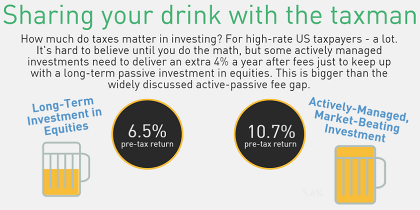
The passive vs active investing debate usually centers on low vs high fees and the plausibility of superior investment performance. For many taxable investors, taxes can matter more than either of those, as there can be a huge difference in the slice of returns you pay in taxes between passive and active investment styles. We put together an infographic to illustrate this difference in a practical example for a US high rate taxpayer.

Assumptions and discussion of other cases:

Tax is a complex topic.¹ Each of us has a different tax situation, and even within a family, different pools of savings are taxed differently. I based this note on the case of a high income US taxable investor, resident in a no-income-tax state (e.g. Texas, Florida, Wyoming). I assume (perhaps optimistically) today’s tax rates, and tax rules, stay constant in the future. Today’s federal tax rates are 39.6% for short-term capital gains and ordinary income, and 20% for long-term capital gains and Qualified Dividends. All investment income is subject to the 3.8% Affordable Health Care tax (aka Obama-care tax).² There are a variety of limitations on deduction of investment related expenses in the tax code, which can make a big difference in after-tax returns. In the base case, I have assumed miscellaneous itemized deductions are only partially disallowed, but I also present the case of full non-deductibility of these expenses.

I’m comparing two fairly extreme cases, but they are not the most extreme I could have chosen. For example, for tax-payers subject to high state taxes the gap would be even greater.

Investment gurus such as Vanguard founder John Bogle and Yale endowment’s David Swenson counsel investors to put their focus on what they can control, and in addition to controlling fees, investors can have quite a lot of control over how their investments are taxed. This is a general note about the impact of taxes on investment returns, and is not specific to any strategy pursued by Elm Partners, although tax awareness is an integral part of our approach. Please feel free to get in touch with me if you’d like more detail or just a general discussion of the topic.

For the Passive Equity Investment, I use 6.5% as the long-term expected return of the global stock market, comprised of an expected real return of 4.5% and expected inflation of 2%. See this video for why 4.5%, but in summary I use 2.5% as the current global stock market dividend yield (it would be about 3% if adjusted for U.S. stock buyback activity) plus an expected real dividend growth rate of 2% (1.5% adjusted for buybacks). For simplicity, I assume all dividends are Qualified Dividends, although for a global equity portfolio this is currently not quite the case.³ I assume that the equity investor uses ETFs to pursue a buy-and-hold strategy, and that ETFs are sufficiently tax efficient that they will not throw off any capital gains (unlike investments in 40 Act mutual funds) even though the underlying indexes on which they are based do produce portfolio turnover (see this note for more on this tax benefit of investing in ETFs). If portfolio turnover were 5% per annum,⁴ the value of deferral would be lower by about 0.1% for a 25 year horizon, and the benefit of an extra 25 years would be about 0.1% lower too.

In the ultimate case of a long-term investment in equities that will be donated or bequeathed at the horizon, the after-tax rate of return is simply the starting dividend rate, after-tax, plus dividend growth, which given the above numbers is:

2.5% * (1 – 23.8%) + 4% = 5.9%

For the generic Actively Managed Investment, I chose a 10.7% pre-tax return so that it results in the same after-tax return of 5.9% enjoyed by the passive investment in equities. I assume the Actively Managed Investment return comes in the form of ordinary income or short-term capital gains. In practice, the tax characteristics of a given actively managed investment may be more attractive than this (e.g. having some component of qualified dividends, long-term capital gains or deferred capital gains), or less attractive (e.g. ones that throw off interest income together with capital losses which cannot be netted against the income⁵). It is worth bearing in mind that many, but not all, active alternative investment vehicles are aimed at institutional investors such as pension funds or endowments which do not pay tax, and hence they may not be managed with tax efficiency a priority. I assume miscellaneous itemized deductions of 2.5% each year (e.g. management fee of 2% plus administration, legal and audit expenses of 0.5%)⁶ In case you’re not familiar with the term “miscellaneous itemized deductions,” think of it as IRS code for “expenses that the tax rules try to prevent you from deducting from your income.” I assume that the tax circumstances of the investor are such that the deduction cannot be taken in full, but are limited by the 2% and 3% of adjusted gross income limitations on deductions and also the disallowance of deductions in the application of the 3.8% Obama-care tax⁷.

How a 10.7% pre-tax return turns into a 5.9% after-tax return is quite straightforward. First, tax the 10.7% return at the 43.4% tax rate, and then subtract the 6.0%⁸ of the 2.5% miscellaneous itemized deduction which is disallowed, so:

10.7% * (1 – 43.4%) – 6.0% * 2.5% = 5.9%

Other cases:

For the base case I used above, I assumed a partial but not total loss of miscellaneous itemized deductions. Many investors have miscellaneous itemized deductions that are less than 2% of adjusted gross income, which means that they are completely disallowed. In such a case, the pre-tax return of an Actively Managed Investment would need to be 12.4% rather than 10.7%, which is nearly double the pre-tax return of a tax-efficient long-term investment in equities:

12.4% * (1 – 43.4%) – 43.4% * 2.5% = 5.9%

Let’s take a look at how these numbers come out for an investor who lives in a state with a high (say 9%, which is close to the top rate in NY State) income tax.

For the long-term, passive equity investor, the marginal tax rate will be roughly:

20% + 3.8% + 9% = 32.8%
(assuming state tax on investment income
isn’t deductible against federal tax)

The after-tax return of a long-term equity investment with this tax rate, taking account of deferral and the benefit of stepped-up basis at the horizon, will be 5.7%, for an effective tax rate of 12%. With 25 years of deferral, but not stepped-up basis benefit, the after-tax return would be 4.9%.

For the Actively Managed Investment, I’ll assume that the investor has enough deductions so that the relevant federal tax rate is the 28% Alternative Minimum Tax (AMT). Note that in the AMT, all deductions (miscellaneous and other, except for charitable contributions) are disallowed. The tax rate here is:

28% + 3.8% + 9% = 40.8%

The return required to deliver the 5.7% after-tax return of long-term equities is 11.3%:

11.3% * (1 – 40.8%) – 40.8% * 2.5% = 5.7%
(a 50.0% effective tax rate)

What return does this active investment need to deliver before fees, assuming it’s an alternative investment with a 20% incentive fee on the return in excess of the 2.5% management and operational fees? The answer is 16.7%, roughly 2.5x the return of a passive long-term investment in equities:

(11.3% + 2.5%) / (1 – 20%) = 16.7%

Investors generally view equities as providing some protection against higher inflation. In our base case, we assumed 2% inflation, and found that Actively Managed Investments needed to return 4.2% more than equities (10.7% vs 6.5%) in order to deliver the same after-tax return. If we assumed inflation of 4%, and a long-term equity return of 8.5% (still a 4.5% real return), an Actively Managed Investment would need to earn 5.7% more than equities (14.2% vs 8.5%) in order to give the same after-tax return. In real terms, an investment in equities may well provide better protection against higher inflation.

I do not show the effects of investment volatility on these tax outcomes. For example, when you pay taxes on your returns in full every year, and then have a loss one year, the government generally doesn’t pay you “negative taxes” – you just have to carry that capital loss forward into the future and hope for better times ahead. If you’ve reached your investment horizon (e.g. you’re donating or gifting your wealth), then you don’t get any benefit of the capital loss. This can be a significant effect⁹. For example, in the case of an investment that has 15% annual volatility and delivers 6% a year annual return, this asymmetry in tax treatment can lead to a drain of about 0.4% a year over a 25 year horizon.

I have left for a future note a discussion of “tax loss harvesting,” which for some investors can be a significant extra benefit of tax-aware investing. I also do not take account of how different investment styles tend to be more or less tax efficient. See this 2012 paper by Israel and Moskowitz for a discussion of why value investing is not very tax efficient, while momentum investing is.

Please feel free to get in touch to discuss further, or to make this note better.

---

Other references:

“Taxman” – The Beetles

---

1. I’d like to thank my friend Larry Hilibrand (like me, not a tax expert), who has very patiently helped me to focus on and understand these issues. If you want expert advice on taxes, you should speak to my accountant, David Untracht – he’s terrific. Of course, any errors in this note are my own.
   
2. This is a simplification. For example, some degree of investment related expenses are allowed as deductions in the computation of the affordable health care tax surcharge.
   
3. Just under 90% of dividends in Vanguard’s global equity ETF, VT, were qualified in 2014.
   
4. And average cost accounting were used instead of specific tax lot accounting.
   
5. Such as may occur with a portfolio of high yield bonds that pay a high rate of interest but suffer occasional realized capital losses from defaults.
   
6. For some investments, the amount of these itemized deductions can be well in excess of 2.5%, such as in private equity or VC vehicles that charge fees on committed, but undrawn capital, or that incur significant portfolio expenses in making their investments.
   
7. I did not take account of the potential benefit that a high return/high tax investment might have in estate planning, for example in a case where a parent, through use of a trust, pays the tax on an investment while giving the return to a beneficiary (in addition to not being a tax expert, I am also not an estate expert).
   
8. 6.0% = 2% of 43.4% + 3% of 43.4% + 3.8%
   
9. There may also be more subtle convexity effects, beyond the scope of this short note, that become apparent in the presence of investment volatility.
   

A few months ago we posted a short video, titled “The Most Important Number You Won’t Find in the Wall Street Journal,” which described a simple way to forecast the long term expected real return of the stock market. The method consisted of adding together the “three easy pieces” of 1) the market’s current dividend yield, plus, 2) expected real dividend growth, plus, 3) an adjustment for any forecast change in stock market valuation. At very long horizons, say 50 years, the adjustment for one’s expected change in stock market valuation has a small impact on expected returns. For global equities, this approach suggests a long-term inflation adjusted expected return of about 4.5% based on current market pricing.

In the video, I showed that this approach gave a good estimate for the two 50 year non-overlapping periods for which we have good stock market data, 1915 to 1965 and 1965 to 2015. I received quite a few comments and questions, with many people asking whether the 1915 and 1965 starting dates were particularly good times for this forecasting method. The chart above addresses this by showing the forecast for the real return of the US stock market on a rolling basis from 1872 to 1965, using data from Professor Robert Shiller’s website (using the last 12 month dividend yield adjusted for the past year’s performance). For roughly 90% of the 1,120 monthly forecasts, the forecast was within 1.5% of the outcome, and 99% of the time, the forecast was within 2.5% of the realized outcome. This is more than twice as accurate as using historical returns to forecast future returns or using a constant 5% real return as the forecast. Not bad for such a simple forecasting method.

Another question concerned the effect of the time horizon on the accuracy of the forecast. As you’d expect, the shorter the time horizon, the less accurate the forecasts from this simple cash-flow based approach. The chart below shows how the accuracy of the forecast goes down with shorter horizons, using just dividend yield and expected dividend growth for our forecast (i.e. not including any adjustment for a view regarding future changes in market valuation). For horizons of less than 25 years, we need the mythical crystal ball, while for longer horizons a pencil and the back of a small envelope will do the job.

Finally, a word on real returns versus nominal returns. Real, inflation-adjusted returns are what will determine our future purchasing power. Fortunately, they are also easier to predict; long term real equity returns have been 20% to 40% less volatile than nominal returns over the past 140 years of US stock market history.

There is a rich academic and practitioner research literature on forecasting stock market returns, which deals more rigorously with the topic and also explores the equity expected returns on an international basis. You’ll find an abbreviated list of some relevant reading below.

---

Note:

This note does not constitute an investment offering, but rather is intended to elicit discussion and exploration of better ways to invest. Simulated historical returns and past performance are not indicative of future results.

---

Further Reading and References:

• John Campbell and Robert Shiller. “Stock Prices, Earnings, and Expected Dividends.” Journal of Finance. July 1988.
• Robert Shiller. Irrational Exuberance. Princeton University Press. 2000.
• Jeremy Siegel. The Shiller CAPE Ratio: A New Look. University of Pennsylvania Working Paper. 2014.
• Brad Delong. “Under what circumstances should you worry that the stock market is ‘too high’.” Brad Delong’s Blog. August 2014.
• Dimson, Marsh, Staunton et al. Research Institute Yearbook. 2015.

The Wall Street Journal publishes 10,000 different numbers every day…but you won’t find the one that’ll help you decide how much to save or how to invest your savings. In this short talk – based on presentations given at MIT, UPenn, Columbia, the LSE and the JH Weds Lunch Club – we’ll show you an easy way to compute this number for yourself.

Assets invested in Exchange Traded Funds (ETFs) just broke through the $3 trillion milestone, 25 years since their birth.¹ At Elm Partners we use ETFs extensively, making up about 40% of our $390mm assets under management. An often quoted advantage of ETFs is that they can be easily traded all day long, rather than once a day at the close as with traditional open-ended mutual funds. At Elm Partners, we invest with a long-term horizon, and we believe that ETFs have at least three less publicized advantages for long-term investors like us, namely: 1) insulation of long-term holders from the trading costs induced by investor turnover, 2) improved tax efficiency, and 3) lower cost structure.

Not everyone is a fan. Critics argue that ETFs are a source of financial instability. Ironically, some of the most strident criticism comes from Jack Bogle and Larry Fink, the founders of the two biggest ETF sponsors, Vanguard and Blackrock. They argue that many of the nearly 6,000 available ETFs do not have the desirable features we should expect from passive, index oriented products, such as low cost, diversification, transparency and simplicity. We agree with this criticism, and avoid ETFs with labels such as “synthetic,” “actively managed,” “leveraged” and “inverse”.

However, we disagree with Bogle when he states that ETFs are “just great big gambling, speculative instruments that have definitely destabilized the market.”² We believe the ETF structure is a source of financial stability, and better for long-term investors, as compared to traditional mutual funds. Here’s why.

Insulating long term investors from costs of subscriptions and redemptions

In a traditional mutual fund, the costs of having to buy or sell securities to accommodate incoming or departing shareholders are borne by the investors who remain in the fund, rather than by the investors who trigger those costs. In normal times, these costs can add up to as much as 0.10% of extra annual cost for long term mutual fund investors.³ However, in times of crisis this flawed design feature is exploited by sophisticated investors who make a concerted rush for the exit, so that they can get out at the mid-market net asset value (NAV) price, leaving the remaining investors to bear the heavy cost of the liquidations they instigated.

By contrast, in an ETF, competing brokers (called Authorized Participants) create and redeem ETF shares in exchange for the basket of individual securities that comprise the ETF.⁴ No trades take place, and hence no costs are incurred, inside the ETF as investors enter or exit. Existing ETF investors are thereby insulated from the costs of buying or selling securities to accommodate subscriptions and redemptions.

In turbulent times, this mechanism protects long-term investors while accommodating investors who want to exit at a fair, non-subsidized price. True, an ETF which is based on underlying assets that are not very liquid, such as high yield bonds, can give investors a false sense of liquidity. If many holders want to sell, not only will the price of the asset class fall dramatically, but the arbitrage mechanism will not stop the price of the ETF going to a substantial discount to NAV, and even to a discount to the bid side of the underlying assets. While this isn’t a pleasant scenario for the holder of that ETF, we think it is much better than what happens with an open-ended mutual fund structure. With ETFs there is no incentive for investors to be first out the door, as each investor bears her own marginal cost of increasing or decreasing the fund size.

Tax efficiency

The second, related, reason we like ETFs is that they are more tax efficient than typical open ended mutual funds.⁵ US mutual fund tax accounting means that realized capital gains caused by redemptions are allocated to all investors who hold the fund at year end, even though those remaining were not responsible for triggering the capital gain. The tax basis of their holding will be increased, so when they eventually redeem, there won’t be a double counting of capital gains, but the acceleration of their tax liability and the potential of being allocated higher-taxed short term capital gains is unpleasant and unfair.

With ETFs, redemptions do not trigger sales that generate capital gains. Instead they cause the fund manager to deliver a basket of the underlying fund assets to the Authorized Participant who in turn gives shares of the ETF to the fund manager for redemption. The tax efficiency can be further enhanced by the fund manager delivering the lowest basis tax lots held inside the fund to the Authorized Participant. The ETF tax advantage, over a long term horizon, can be worth as much as an extra 0.5% of annual return on an after-tax basis for US taxable investors.⁶ ETFs tend to be more tax efficient than their mutual fund counterparts for non-US offshore investors too. For example, the withholding tax rate on Irish listed ETFs that invest in US equities is 15%, as compared to 30% for comparable Irish listed mutual funds.

Cost efficiency

Finally, ETFs are typically cheaper to run than mutual funds, and this cost saving tends to get passed on to investors. ETFs usually have lower marketing, distribution, accounting and administration (including KYC and AML) expenses. This probably explains why Vanguard charges higher fees on its mutual funds than it does on its ETFs.⁷ Many ETF trades do not trigger a subscription or redemption with the related trades in the basket of securities underlying the ETF. Rather they can be traded between a buyer and seller of the ETF itself. These direct trades in the ETF, bypassing the basket, are referred to as the “ETF liquidity layer,” which can lead to an ETF trading at a much tighter bid-offer spread than the underlying market, thus reducing the total cost of investor turnover.

Investing in an ETF does involve paying the bid-offer spread, and there’s also the risk that the price of the ETF declines in relation to NAV. These and other considerations mean that, contrary to the conventional view, an investor with a short term horizon may actually prefer going in and out of a mutual fund at NAV as compared to trading the ETF. You will see from our monthly portfolio reports on our website that we continue to use traditional mutual funds in many cases.

So where does this leave us? Perhaps the most broadly voiced criticism of ETFs remains so far unanswered: that they tempt investors to become active, short term traders, which has been shown to cost investors a lot in the long term. Jack Bogle is joined by Warren Buffett, the Bank of England’s Andrew Haldane and many others on this one. Responding to their founder’s concerns, the researchers at Vanguard wrote a report, aptly titled, “ETFs: For the Better or the Bettor?” (July 2012). While we’d like to see all investors succeed (we are not engaged in zero sum investment management), we agree with the Vanguard researchers’ conclusion that the temptation effect “is not a reason for long-term individual investors to avoid using appropriate ETF investments as part of a diversified investment portfolio.”

We realize we have only scratched the surface of this topic, but we hope we have given you a different perspective on the ETF structure than the conventional view. We hope you’ll agree that the ETF is a valuable financial innovation that is of great benefit to long term investors like us.

Please feel free to get in touch to share your thoughts or to delve more deeply into ours.

---

For more information about Elm Partners and our investment strategy, please visit us at ElmWealth.com or e-mail info@elmwealth.com.

---

1. Globally, including ETPs, according to www.ETFGI.com. For simplicity in this note, we’ll use the term ETF to include ETPs in terms of overall marketplace description.
   
2. Zweig, 2011.
   
3. For example, for a fund with 50% annual unmatched investor turnover (which can include net subscriptions), and underlying assets with a 0.20% average bid-ask spread.
   
4. The sponsor can also accept cash or partial baskets, and if the sponsor is not careful, some of the costs can slip into the ETF. Generally, we’ve found that for the biggest ETF sponsors, they are very careful. Also, we should mention that many of Vanguard’s US listed ETFs are a hybrid structure, which has features of both a mutual fund and an ETF. A detailed treatment of this hybrid structure is beyond the scope of this short note.
   
5. We are not offering tax advice. Please consult your tax advisor.
   
6. Based on a 24.4% effective marginal tax rate for long-term capital gains, a 3% dividend yield and long-term growth of 3.5% pa.
   
7. This is generally the case for Vanguard’s US listed Investor shares vs ETFs, and also the case for their Irish listed fund and ETF products.
   

Each of our strategies follows our rules-based asset allocation methodology, an approach we call Active Index Investing®. This note describes in detail the three main components of this approach: the construction of the Baseline portfolio and the value and momentum overlays to that Baseline portfolio which make the portfolio responsive to changing market conditions.

Throughout this discussion, we will use our Global Balanced Portfolio for US taxable investors as an example and refer to Table 1 below, which is a snapshot of our signals at the end of March 2015. We publish this information every month on our website and intra-month data is available on request.

Table 1: Asset Allocation Table

Risk Level

For each of our strategies, the starting point is to choose the desired level of risk in terms of an equity / fixed income portfolio. For our balanced global asset allocation for US investors, we use a 65%/35% split: 65% global market cap weighted equities, and 35% in US fixed income and money market investments. We expect this to remain constant throughout the life of the strategy.

We do not benchmark ourselves against this portfolio in the traditional sense, in that it plays no role in portfolio management decisions, but instead it can be used by investors as a potentially helpful reference point to provide a context for the targeted risk level of the portfolio and long term return expectations.

Baseline Portfolio

Based on the targeted risk level as described above, we construct our Baseline Portfolio, which is comprised of approximately 20 asset buckets (as listed in the first column of Table 1).¹ The Baseline Portfolio is not market cap weighted. It is constructed to be more balanced and diversified, with exposure to more sources of return, than the more traditional 65/35 equity/fixed income portfolio.

We believe that slavishly relying on market capitalization weights of public market equities published by providers such as MSCI and FTSE is an approach that can be improved upon. Taking account of other considerations (such as GDP, population and corporate earnings) leads to a more diversified and balanced portfolio which is more representative of all global risk assets, public and private. Such a portfolio will better approximate market cap weights in the long-term future with fairly valued markets. This approach mitigates “the tyranny of indexing” by tempering the high weights given to markets with relatively high valuations (recall that the Japanese equity market in 1989 represented 40% of a global market-cap weighted equity index).

We begin by calculating the target regional weights that we will apply to our risk asset allocations. Table 2, below, illustrates our quantitative approach to determining these weights. We give equal weight to market capitalization, cyclically adjusted corporate earnings, population and GDP for each regional equity market. As developing economies (EM) represent 86% of world population and 43% of world GDP, this approach results in a desired weight of nearly 40% to EM. We feel that this would be too much of a deviation from a conventional balanced world portfolio, and so we apply a cap and a floor to all regions limiting their weights to a maximum of two times, or a minimum of one half, their market capitalization weights. These constraints are currently binding only in the case of EM, capped at 19.6%.

As this strategy is structured for US investors, we incorporate a “home bias,” reflecting the greater relevance of US equities to US investors, for example in terms of future consumption. We have set the home bias factor at 1.5 for the US, and between 1.0 and 1.15 for other regional markets.

Table 2: Regional Weight Target Calculations

Once we have calculated our desired regional weights, we then decide what other sources of return to add to the portfolio. For our US global balanced fund, we add real estate assets (e.g. US publicly traded REITs), credit (mostly in the form of high yield bonds), and a tilt of the equity holdings towards small cap and value stocks. Each of these asset classes is very large. For example, the market value of privately held real estate and known oil reserves are each in excess of the total market cap of global public equity markets. So how do we assign weights to these asset classes in our portfolio? Again, we feel that mechanically using the market value of these asset classes does not make sense. We opt for what we consider a practical approach of assigning weights to these assets that are large enough to matter, but small enough so that we can live with them even through periods of underperformance. You will see that these buckets have weights in the range of 2.5% to 5% of the portfolio.

The final step in deriving the Baseline portfolio is to take account of each of these extra asset buckets in the regional weighting scheme. For example, we count the 5% US REIT bucket as part of our US regional bucket, and we count US High Yield in that same US regional bucket, but with a weight of 50%, as we feel that US high yield is about half as risky as US equities. You can see the resultant Baseline Portfolio in Table 1. We expect our Baseline portfolio to change very little year to year, but we do periodically review the line-up (at least annually) and may add or remove asset classes based on the availability of low-cost and liquid investment vehicles. You can find a slightly more detailed description of this process in our December 2014 monthly report.

Rebalancing Methodology

Each of Elm’s strategies has a prescribed rebalancing methodology. In this example, we rebalance the portfolio at the end of each month and calculate the set of desired deviations from each Baseline asset bucket weight based on our valuation and momentum overlays. Overall, depending on our valuation and momentum adjustments, each asset bucket can go down to an allocation of zero or can be twice that of its Baseline weight, subject to our no-leverage constraint.

Valuation Overlay

For each asset bucket, we use a simple valuation metric, such as cyclically adjusted earnings yield for equity buckets, as a signal of whether that asset bucket is over- or under-valued. We determine fair value for each bucket, based on what we think is a fair forward-looking expected return. For example, for most equity buckets, we believe a 6% earnings yield is about fair, as we think it is consistent with about a 4-5% long-term real return on equities. We strive to keep our approach as simple as possible, and so the desired deviation from the Baseline weight for each bucket is generally proportional to how far from fair value that asset class is currently priced. Backward-looking optimization is not part of the process.

Now let’s take a closer look at the row for US REITs (our valuation measures are the orange columns).

You can see that the Baseline weight is 5% and the valuation measure we use is the 10 year inflation-adjusted dividend yield. We think a 6% dividend yield is fair value in that we feel it is consistent with a 4-5% long-term real return. We believe that REIT dividends should keep up with inflation, but that part of the dividend represents a return of capital. We use 6% as our REIT fair value center point. As you can see in the column titled ‘valuation signal’, REITs at the time the table was compiled were trading at a dividend yield of just 3.5%. This is around 40% lower than our fair value center point (54% lower on a log scale, which we find a slightly more consistent way to measure the deviation, as it doesn’t matter which number we chose to be the numerator or denominator of the ratio). So, we want 54% less of that 5% REIT bucket from a valuation point of view, which is 2.7% less.

We limit the deviation we allow based on valuation to 2/3 of the asset bucket’s Baseline Weight, which is not a constraint in this particular case.

Certain asset buckets are treated as sub-buckets, which are indented in table. We use a relative valuation metric to decide how much of that asset class we desire to hold in the form of the sub-bucket. For example, this is how we decide on the weight of US small caps within the overall US equity bucket, or municipal bonds within the US fixed income bucket.

Momentum Overlay

For each asset bucket we then compute a simple momentum measure, which compares the current value of that asset to its average over the past 12 months. We do this taking account of inflation, dividends and risk premium, so that the momentum signal is as likely to be positive as negative, and so does not give us a bias to be overweight our asset buckets versus the Baseline weights.

Unlike our valuation overlay, our momentum overlay is binary, so for an asset bucket that has negative momentum, we desire 1/3 less than its Baseline weight, and for positive momentum, we desire 1/3rd more of that bucket. However, we do establish a narrow transition zone across which the momentum adjustment goes from -1/3rd to +1/3rd, so that the signal is not completely binary. For example, for US REITs, the transition zone is +-2.5%. This transition zone helps us to reduce portfolio turnover and transactions costs.

Again looking at the row for US REITs (our momentum measures are in the blue columns), you can see that in this example US REITs had positive momentum of 9.5%, and so we desire 1/3 more than the 5% Baseline weight, or 1.7% more.

In the case of sub-buckets (indented in the table), such as the US small cap bucket, we follow the same process as for the valuation overlay, applying the momentum overlay on a relative basis, to determine how much of the higher level bucket should be held in the form of the sub-bucket.

Putting it all together: Desired Portfolio Weights

Then, for each asset bucket we simply add the valuation adjustment to the momentum adjustment to get the total desired deviation for that bucket. For US REITs, that number is -1.0% (-2.7% + 1.7%, with a little bit of rounding).

As valuation can only change the bucket by +-2/3rds and the momentum adjustment by +-1/3rd, the desired weight for a bucket will be between 0 and two times its Baseline weight.

We then add up all the desired weights of all the asset buckets, except for the Cash bucket. If the weights add up to less than 100%, then we are finished, and the remainder is the Cash bucket allocation. If, however, the weights add up to more than 100%, then we divide each weight by the sum of the weights and these scaled down weights become the desired weights for each bucket. They will add up to 100% and the Cash bucket will be 0.

History

Over the history of our global balanced portfolio for US taxable investors, the Cash bucket has not yet been zero, but has ranged between 11% and 48%. On a simulated basis it reached a level of 67% in July 2008 and zero in August 2009 (although you cannot see this in Chart 1 below as data is shown every six months).

Chart 1 below shows how the desired asset allocation has changed over the life of our Fund (January 2012), and prior to that back to the start of 2007 (on a simulated basis prior to 2012). In separate back-tests from 1925 and 1975 to the present, the value and momentum dynamic asset allocation approach described in this note improved investment returns and decreased risk as compared to a comparable static Baseline portfolio. For more detail, please see the research note, “Investing for the Rest of Us.”

Chart 1: Historical Asset Allocation

At least once a year, we review our investment approach in detail, and consider improvements. We favor those that make our approach simpler and more intuitively appealing, which we hope will help us stay the course for the long term, and prevent ad hoc, subjective views making an unwanted entry into our process.

We hope this description of our methodology has left you with a clearer understanding of how we implement our Active Index Investing® approach. We have tried to go into enough detail so you can understand every aspect of our methodology, but please don’t hesitate to get in touch with any questions or suggestions you may have. We value your input.

---

Disclaimer:

The information contained on this page has been provided as general commentary and for information purposes only. It does not constitute any form of advice nor recommendation to buy or sell any securities or adopt any investment strategy mentioned therein. It is intended only to provide observations and views of the author(s) at the time of writing, both of which are subject to change at any time without prior notice. The information contained in the commentaries is derived from sources deemed by Elm Partners to be reliable but its accuracy and completeness cannot be guaranteed. This material does not have regard to specific investment objectives, financial situation and the particular needs of any specific person who may read it. It is directed only at professional investors as defined by the rules of the relevant regulatory authority. Any views regarding future prospects may or may not be realized. Past performance is no guarantee of future results.

---

1. Notice that the allocation to fixed income and cash in the Baseline portfolio is 25% as compared to 35% in the 65/35 simple target portfolio. The reasons for this are: 1) the Baseline is a more diversified and balanced portfolio and so should be able to support a smaller weight in fixed income and cash, and 2) as described below, our dynamic asset allocation approach can reduce risk more than it can increase it, due to our leverage constraint.
   

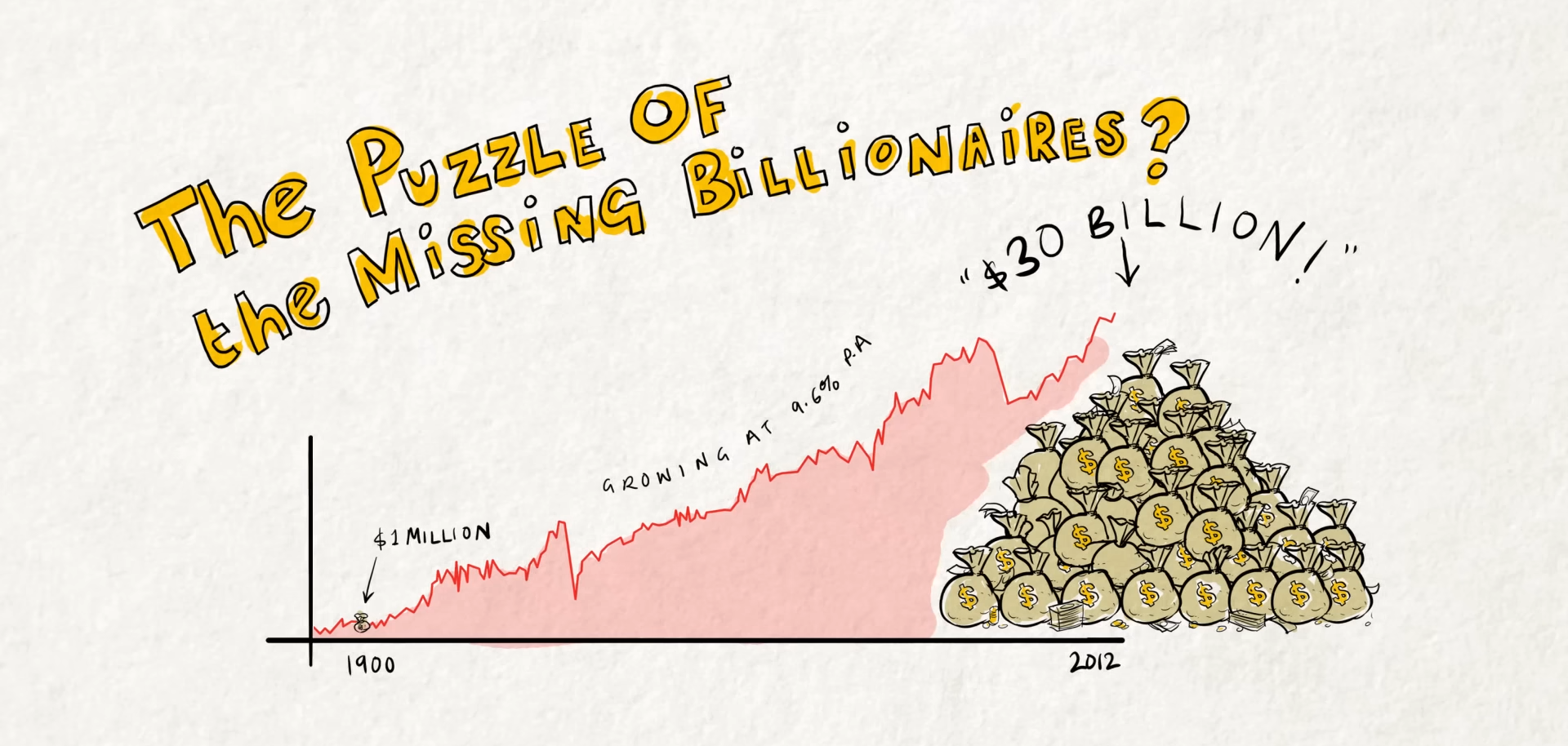
In this TEDx talk (which has over 190,000 views as of 2024), I use the puzzle of the missing billionaires to explore how and why most investors fail to capture the returns offered by the market.

I try to put forward a simple but powerful solution for those who aren’t satisfied with the status quo: it’s called Active Index Investing®. This approach combines the best features of low-cost index funds with the appealing and successful aspects of active management.